setwd("C:/Desktop/DSR/Session 3")Exercise 1: Covid-19 and global income inequality (Deaton)
Session 3
Download datasets on your computer
Put them a subfolder called data in your working directory.
Load data and install useful packages
First, set your working directory:
library(tidyverse) # {dplyr}, {ggplot2}, {readxl}, {stringr}, {tidyr}, etc.library(ggplot2) repository <- "data"# COVID-19 deaths data: read CSV file, using Windows ISO-8859-1 Latin-1 encoding
deaths <- readr::read_csv(
paste0(repository, "/covid-deaths-daily-vs-total-per-million.csv"),
locale = locale(encoding = "latin1"))Rows: 55193 Columns: 7
── Column specification ────────────────────────────────────────────────────────
Delimiter: ","
chr (3): Entity, Code, Continent
dbl (3): Year, Total confirmed deaths due to COVID-19 per million people, D...
date (1): Date
ℹ Use `spec()` to retrieve the full column specification for this data.
ℹ Specify the column types or set `show_col_types = FALSE` to quiet this message.# Population data: read Excel file, skipping first 2 rows
pop <- readxl::read_excel(paste0(repository,
"/API_SP.POP.TOTL_DS2_en_excel_v2_1926530.xls"),
skip = 2)
# read Excel file, skipping first 2 rows
gdpc <- readxl::read_excel(paste0(repository,
"/API_NY.GDP.PCAP.PP.KD_DS2_en_excel_v2_1930672.xls"),
skip = 2)Prepare COVID-19 deaths data
Clue
See dplyr::filter and as.Date()
Solution
deaths <- deaths %>%
  filter(Date <= as.Date("2020-12-31"))
Clue
See dplyr::group_by and dplyr::filter and use them one after each other using the max function inside to get the latest date.
Solution
deaths <- deaths %>%
  group_by(Code) %>%
  filter(Date == max(Date))
Clue
See dplyr::select.
Solution
deaths <- deaths %>%
  select(
    country = Entity,
    ccode = Code,
    date = Date,
    deaths = "Total confirmed deaths due to COVID-19 per million people"
  )
Note the quotes, which are required to select columns when their names include spaces or other special characters, such as ‘.’. You can you double quotes, simple quotes and even backticks.
Clue
See dplyr::mutate to create or transform a variable and the log function inside.
Solution
deaths <- deaths %>%
  mutate(log_deaths = log(deaths))
Prepare population data
Clue
See previous questions! You’ll do the same things!
Solution
pop <- pop %>%
  select(
    country = "Country Name",
    ccode = "Country Code",
    pop2019 = "2019"
  ) %>%
  mutate(log_pop = log(pop2019))
head(pop)
# A tibble: 6 × 4
country ccode pop2019 log_pop
<chr> <chr> <dbl> <dbl>
1 Aruba ABW 106314 11.6
2 Afghanistan AFG 38041754 17.5
3 Angola AGO 31825295 17.3
4 Albania ALB 2854191 14.9
5 Andorra AND 77142 11.3
6 Arab World ARB 427870270 19.9Prepare population GDP/capita data
Same steps as above:
gdpc <- gdpc %>%
  select(
    country = "Country Name",
    ccode = "Country Code",
    gdpc2019 = "2019"
  ) %>%
  mutate(log_gdpc = log(gdpc2019))
Merge all data sources and finalise dataset
We will start to see here how we merge two different datasets together.
To merge WDI indicators together, we perform below a ‘full join’ that will keep all observations from both datasets, and there are two identifier variables (country and ccode).
wdi <- full_join(pop, gdpc, by = c("country", "ccode"))
head(wdi)
# A tibble: 6 × 6
country ccode pop2019 log_pop gdpc2019 log_gdpc
<chr> <chr> <dbl> <dbl> <dbl> <dbl>
1 Aruba ABW 106314 11.6 NA NA
2 Afghanistan AFG 38041754 17.5 2065. 7.63
3 Angola AGO 31825295 17.3 6670. 8.81
4 Albania ALB 2854191 14.9 13965. 9.54
5 Andorra AND 77142 11.3 NA NA
6 Arab World ARB 427870270 19.9 14603. 9.59Note: see what happens if you leave out one of the identifying columns/variables
full_join(pop, gdpc, by = "country") %>% head()# A tibble: 6 × 7
country ccode.x pop2019 log_pop ccode.y gdpc2019 log_gdpc
<chr> <chr> <dbl> <dbl> <chr> <dbl> <dbl>
1 Aruba ABW 106314 11.6 ABW NA NA
2 Afghanistan AFG 38041754 17.5 AFG 2065. 7.63
3 Angola AGO 31825295 17.3 AGO 6670. 8.81
4 Albania ALB 2854191 14.9 ALB 13965. 9.54
5 Andorra AND 77142 11.3 AND NA NA
6 Arab World ARB 427870270 19.9 ARB 14603. 9.59To merge WDI indicators to Covid-19 deaths, we perform below an ‘inner join’ that will keep only observations present in both datasets, with identical country names and country codes.
d <- inner_join(deaths, wdi, by = c("country", "ccode"))
head(d)
# A tibble: 6 × 9
# Groups: ccode [6]
country ccode date deaths log_deaths pop2019 log_pop gdpc2019 log_gdpc
<chr> <chr> <date> <dbl> <dbl> <dbl> <dbl> <dbl> <dbl>
1 Afghanis… AFG 2020-12-31 56.3 4.03 3.80e7 17.5 2065. 7.63
2 Albania ALB 2020-12-31 410. 6.02 2.85e6 14.9 13965. 9.54
3 Algeria DZA 2020-12-31 62.8 4.14 4.31e7 17.6 11511. 9.35
4 Andorra AND 2020-12-31 1087. 6.99 7.71e4 11.3 NA NA
5 Angola AGO 2020-12-31 12.3 2.51 3.18e7 17.3 6670. 8.81
6 Antigua … ATG 2020-12-31 51.1 3.93 9.71e4 11.5 21910. 9.99See which rows of deaths have no match in wdi:
anti_join(deaths, wdi, by = c("country", "ccode"))# A tibble: 21 × 5
# Groups: ccode [21]
country ccode date deaths log_deaths
<chr> <chr> <date> <dbl> <dbl>
1 Bahamas BHS 2020-12-31 432. 6.07
2 Brunei BRN 2020-12-31 6.86 1.93
3 Cape Verde CPV 2020-12-31 203. 5.31
4 Congo COG 2020-12-31 19.6 2.97
5 Czechia CZE 2020-12-31 1081. 6.99
6 Democratic Republic of Congo COD 2020-12-31 6.60 1.89
7 Egypt EGY 2020-12-31 74.6 4.31
8 Gambia GMB 2020-12-31 51.3 3.94
9 Iran IRN 2020-12-31 657. 6.49
10 Kosovo OWID_KOS 2020-12-31 689. 6.54
# ℹ 11 more rowsSee which rows of wdi have no match in deaths:
anti_join(wdi, deaths, by = c("country", "ccode"))# A tibble: 109 × 6
country ccode pop2019 log_pop gdpc2019 log_gdpc
<chr> <chr> <dbl> <dbl> <dbl> <dbl>
1 Aruba ABW 106314 11.6 NA NA
2 Arab World ARB 427870270 19.9 14603. 9.59
3 American Samoa ASM 55312 10.9 NA NA
4 Bahamas, The BHS 389482 12.9 37101. 10.5
5 Bermuda BMU 63918 11.1 81798. 11.3
6 Brunei Darussalam BRN 433285 13.0 62100. 11.0
7 Bhutan BTN 763092 13.5 11832. 9.38
8 Central Europe and the Baltics CEB 102378579 18.4 32710. 10.4
9 Channel Islands CHI 172259 12.1 NA NA
10 Congo, Dem. Rep. COD 86790567 18.3 1098. 7.00
# ℹ 99 more rowsBy merging on country names and country codes, we assumed that all three data sources used the same country names and codes… which might or might not be the case: as you can see, COD (Democratic Republic of Congo) gets dropped due to a mismatched country name. This is good enough for our purposes, but a safer and better merge would have used only country codes, and would have harmonised those first with the help of the {countrycode} package, for instance, plus some manual checks.
Lesson: spend enough time learning about your data
Inspect result
You should be checking your results from time to time, either visually, as shown here, or through more thorough/systematic checks
# Open dataset in the viewer
View(d)
# check the first rows
head(d)# A tibble: 6 × 9
# Groups: ccode [6]
country ccode date deaths log_deaths pop2019 log_pop gdpc2019 log_gdpc
<chr> <chr> <date> <dbl> <dbl> <dbl> <dbl> <dbl> <dbl>
1 Afghanis… AFG 2020-12-31 56.3 4.03 3.80e7 17.5 2065. 7.63
2 Albania ALB 2020-12-31 410. 6.02 2.85e6 14.9 13965. 9.54
3 Algeria DZA 2020-12-31 62.8 4.14 4.31e7 17.6 11511. 9.35
4 Andorra AND 2020-12-31 1087. 6.99 7.71e4 11.3 NA NA
5 Angola AGO 2020-12-31 12.3 2.51 3.18e7 17.3 6670. 8.81
6 Antigua … ATG 2020-12-31 51.1 3.93 9.71e4 11.5 21910. 9.99# check the last rows
tail(d)# A tibble: 6 × 9
# Groups: ccode [6]
country ccode date deaths log_deaths pop2019 log_pop gdpc2019 log_gdpc
<chr> <chr> <date> <dbl> <dbl> <dbl> <dbl> <dbl> <dbl>
1 United … USA 2020-12-31 1045. 6.95 3.28e8 19.6 62530. 11.0
2 Uruguay URY 2020-12-31 52.1 3.95 3.46e6 15.1 21561. 9.98
3 Uzbekis… UZB 2020-12-31 18.3 2.91 3.36e7 17.3 6999. 8.85
4 Vietnam VNM 2020-12-31 0.36 -1.02 9.65e7 18.4 8041. 8.99
5 Zambia ZMB 2020-12-31 21.1 3.05 1.79e7 16.7 3470. 8.15
6 Zimbabwe ZWE 2020-12-31 24.4 3.20 1.46e7 16.5 2836. 7.95# another way to check on your dataset, as provided by the {dplyr} package
glimpse(d)Rows: 155
Columns: 9
Groups: ccode [155]
$ country <chr> "Afghanistan", "Albania", "Algeria", "Andorra", "Angola", "…
$ ccode <chr> "AFG", "ALB", "DZA", "AND", "AGO", "ATG", "ARG", "ARM", "AU…
$ date <date> 2020-12-31, 2020-12-31, 2020-12-31, 2020-12-31, 2020-12-31…
$ deaths <dbl> 56.283, 410.383, 62.849, 1087.168, 12.323, 51.058, 956.837,…
$ log_deaths <dbl> 4.030393, 6.017091, 4.140735, 6.991331, 2.511467, 3.932962,…
$ pop2019 <dbl> 38041754, 2854191, 43053054, 77142, 31825295, 97118, 449387…
$ log_pop <dbl> 17.45419, 14.86430, 17.57794, 11.25340, 17.27577, 11.48368,…
$ gdpc2019 <dbl> 2065.036, 13965.349, 11510.557, NA, 6670.332, 21910.185, 22…
$ log_gdpc <dbl> 7.632903, 9.544334, 9.351020, NA, 8.805425, 9.994707, 10.00…# another way yet, provided by base R, which will reveal technical details
str(d)gropd_df [155 × 9] (S3: grouped_df/tbl_df/tbl/data.frame)
$ country : chr [1:155] "Afghanistan" "Albania" "Algeria" "Andorra" ...
$ ccode : chr [1:155] "AFG" "ALB" "DZA" "AND" ...
$ date : Date[1:155], format: "2020-12-31" "2020-12-31" ...
$ deaths : num [1:155] 56.3 410.4 62.8 1087.2 12.3 ...
$ log_deaths: num [1:155] 4.03 6.02 4.14 6.99 2.51 ...
$ pop2019 : num [1:155] 38041754 2854191 43053054 77142 31825295 ...
$ log_pop : num [1:155] 17.5 14.9 17.6 11.3 17.3 ...
$ gdpc2019 : num [1:155] 2065 13965 11511 NA 6670 ...
$ log_gdpc : num [1:155] 7.63 9.54 9.35 NA 8.81 ...
- attr(*, "groups")= tibble [155 × 2] (S3: tbl_df/tbl/data.frame)
..$ ccode: chr [1:155] "AFG" "AGO" "ALB" "AND" ...
..$ .rows: list<int> [1:155]
.. ..$ : int 1
.. ..$ : int 5
.. ..$ : int 2
.. ..$ : int 4
.. ..$ : int 148
.. ..$ : int 7
.. ..$ : int 8
.. ..$ : int 6
.. ..$ : int 9
.. ..$ : int 10
.. ..$ : int 11
.. ..$ : int 25
.. ..$ : int 16
.. ..$ : int 18
.. ..$ : int 24
.. ..$ : int 13
.. ..$ : int 23
.. ..$ : int 12
.. ..$ : int 20
.. ..$ : int 15
.. ..$ : int 17
.. ..$ : int 19
.. ..$ : int 22
.. ..$ : int 14
.. ..$ : int 21
.. ..$ : int 28
.. ..$ : int 27
.. ..$ : int 138
.. ..$ : int 30
.. ..$ : int 31
.. ..$ : int 35
.. ..$ : int 26
.. ..$ : int 32
.. ..$ : int 33
.. ..$ : int 34
.. ..$ : int 37
.. ..$ : int 38
.. ..$ : int 54
.. ..$ : int 40
.. ..$ : int 39
.. ..$ : int 41
.. ..$ : int 3
.. ..$ : int 42
.. ..$ : int 45
.. ..$ : int 133
.. ..$ : int 46
.. ..$ : int 48
.. ..$ : int 50
.. ..$ : int 49
.. ..$ : int 51
.. ..$ : int 52
.. ..$ : int 149
.. ..$ : int 53
.. ..$ : int 55
.. ..$ : int 58
.. ..$ : int 59
.. ..$ : int 44
.. ..$ : int 56
.. ..$ : int 57
.. ..$ : int 60
.. ..$ : int 62
.. ..$ : int 36
.. ..$ : int 61
.. ..$ : int 63
.. ..$ : int 66
.. ..$ : int 65
.. ..$ : int 68
.. ..$ : int 67
.. ..$ : int 64
.. ..$ : int 69
.. ..$ : int 70
.. ..$ : int 71
.. ..$ : int 73
.. ..$ : int 72
.. ..$ : int 74
.. ..$ : int 75
.. ..$ : int 76
.. ..$ : int 78
.. ..$ : int 80
.. ..$ : int 81
.. ..$ : int 82
.. ..$ : int 134
.. ..$ : int 79
.. ..$ : int 83
.. ..$ : int 84
.. ..$ : int 77
.. ..$ : int 98
.. ..$ : int 95
.. ..$ : int 94
.. ..$ : int 85
.. ..$ : int 88
.. ..$ : int 93
.. ..$ : int 108
.. ..$ : int 89
.. ..$ : int 90
.. ..$ : int 100
.. ..$ : int 97
.. ..$ : int 96
.. ..$ : int 99
.. .. [list output truncated]
.. ..@ ptype: int(0)
..- attr(*, ".drop")= logi TRUELook how you identify OECD countries
oecd <- c("AUS", "AUT", "BEL", "CAN", "CHL", "CZE", "DNK", "EST", "FIN",
          "FRA", "DEU", "GRC", "HUN", "ISL", "IRL", "ISR", "ITA", "JPN",
          "KOR", "LVA", "LTU", "LUX", "MEX", "NLD", "NZL", "NOR", "POL",
          "PRT", "SVK", "SVN", "ESP", "SWE", "CHE", "TUR", "GBR", "USA")

d$oecd <- d$ccode %in% oecd
head(d[, c("oecd", "ccode")])
# A tibble: 6 × 2
# Groups: ccode [6]
oecd ccode
<lgl> <chr>
1 FALSE AFG
2 FALSE ALB
3 FALSE DZA
4 FALSE AND
5 FALSE AGO
6 FALSE ATG Note: the steps from that section and the previous one could have been written as a single sequence of instructions:
 full_join(pop, gdpc, by = c("country", "ccode")) %>%
   inner_join(deaths, by = "ccode") %>%
   mutate(oecd = ccode %in% oecd)
Visualize
{ggplot2} plot syntax is the topic of our next session together, so feel free to just ignore the code above when revising what we learnt today
But if you are interested, see how to redraw Deaton’s Fig. 1, or at least something close enough to it.
ggplot(d, aes(x = log_gdpc, y = log_deaths, color = oecd, size = pop2019)) +
  # label China and India
  geom_text(
    data = filter(d, ccode %in% c("CHN", "IND")),
    aes(label = country, color = oecd),
    size = 5
  ) +
  # draw linear trend
  geom_smooth(
    method = "lm", mapping = aes(color = NULL, weight = pop2019), se = FALSE,
    lty = "dashed", size = 2/3
  ) +
  # draw actual data points
  geom_point(shape = 1, stroke = 1) +
  # control colours
  scale_color_manual(values = c("TRUE" = "black", "FALSE" = "#aa0000")) +
  # control point size
  scale_size_continuous(range = c(2, 20)) +
  # final cosmetics
  theme_light() +
  theme(legend.position = "none", panel.grid.minor = element_blank())
Warning: Using `size` aesthetic for lines was deprecated in ggplot2 3.4.0.
ℹ Please use `linewidth` instead.`geom_smooth()` using formula = 'y ~ x'Warning: Removed 8 rows containing non-finite outside the scale range
(`stat_smooth()`).Warning: Removed 8 rows containing missing values or values outside the scale range
(`geom_point()`).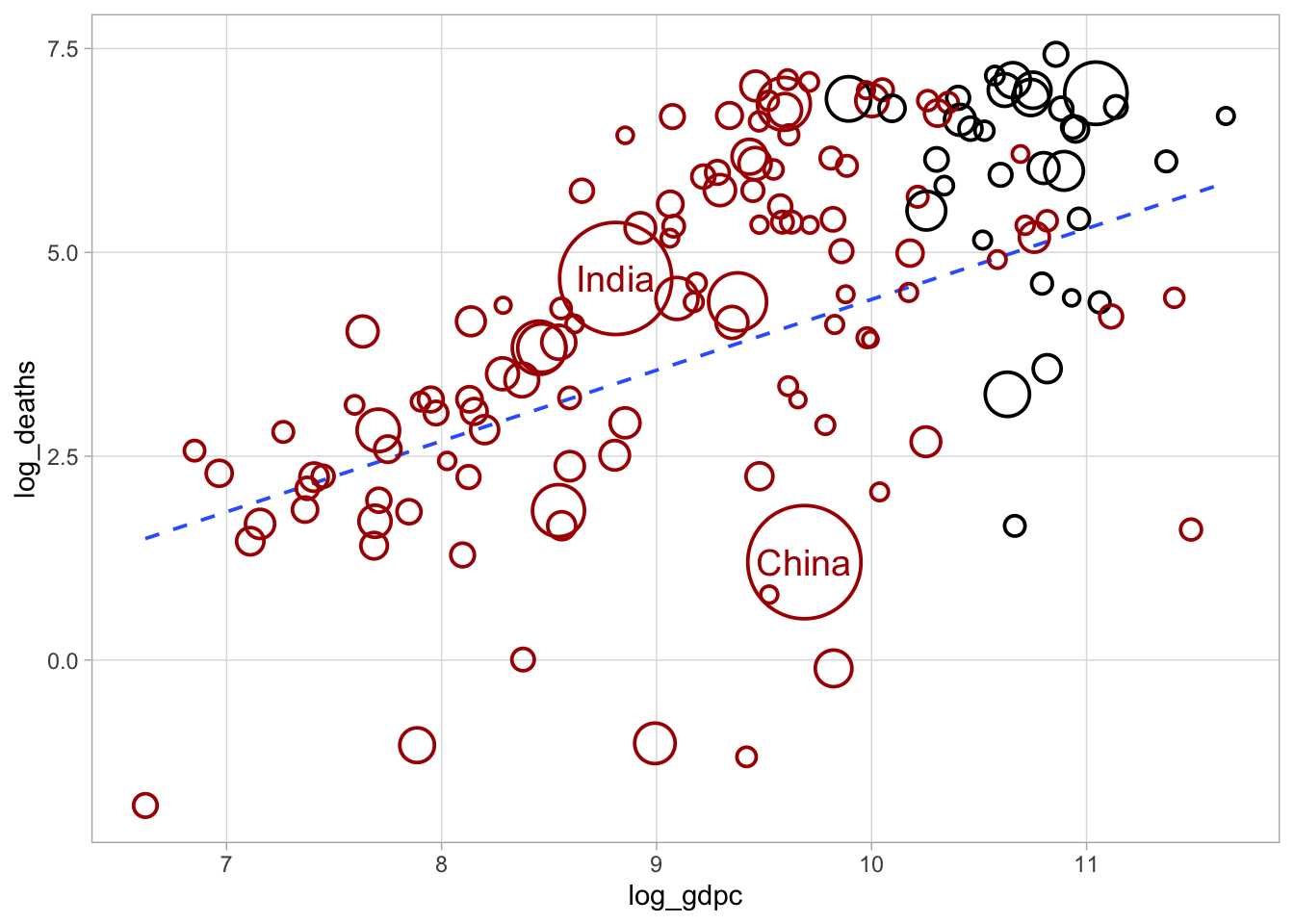
Source
Inspiration
Angus Deaton, “COVID-19 and Global Income Inequality”, working paper, January 2021. Later published on that same year as NBER Working Paper No. 28392, and then as an article in the LSE Public Policy Review 1(4): 1-10.
Data sources
Data source for Covid-19 deaths:
“Daily vs. Total confirmed COVID-19 deaths per million,” Our World in Data, as provided in early 2021.
At the time of download, Our World in Data was sourcing its raw data from the COVID-19 Data Repository by the Center for Systems Science and Engineering (CSSE) at Johns Hopkins University.
See the Our World in Data website for an updated Covid-19 dataset.
Data source for income and population:
World Bank World Development Indicators. The indicators were downloaded manually in February 2021; more recent data can be downloaded through the WDI package.
Data source for OECD member states:
C.J. Yetman, memberstates: List of member states of various international organizations, R package version 0.0.0.9000.
The code to extract and prepare the country code follows:
library(countrycode)
library(memberstates) # remotes::install_github("cjyetman/memberstates")

memberstates::memberstates$oecd$iso3c %>%
  countrycode::countrycode("iso3c", "wb") %>%
  dput()