Exam 1: Road traffic accidents in France [data cleaning and analysis]

For March, 12th

Authors

Kim Antunez

In this exam, you will explore a real-world dataset containing information about road traffic accidents in France in 2022. You’ll perform data cleaning and data analysis tasks to gain insights from the dataset.

You will be assessed on your ability to manipulate the dataset, apply relevant analysis techniques, and communicate your findings effectively.

This is a graded exercise, to be completed in groups. Make sure to adhere to all ethical and academic integrity standards.

Task 1: Data Preparation

Download datasets

The Etalab database of French road traffic injury accidents for a given year is divided into 4 sections, each represented by a CSV file:

The CARACTERISTIQUES (CHARACTERISTICS) section that describes the general circumstances of the accident.
The LIEUX (LOCATIONS) section that describes the main location of the accident, even if it occurred at an intersection.
The involved VEHICULES (VEHICLES) section.
The involved USAGERS (USERS) section.

Download two datasets here:

usagers-2022.csv
carcteristiques-2022.csv [be careful of the typo (carc instead of caract)]

Question 1

First, as usual, set your working directory in R and put the downloaded datasets in a data folder.

Then, load the required packages and the datasets into R.

BE CAREFUL of the unusual delimiter ; in French datasets, instead of ,. See the parameter delim in ?readr::read_delim instead of the usual readr::read_csv.

Don’t worry about the following warning for the moment: Warning: One or more parsing issues, call problems() on your data frame for details.

Solution

library(tidyverse) # of simply {dplyr}, {readr}, {ggplot2}.

repository <- "data"

users <- readr::read_delim(paste0(repository, "/usagers-2022.csv"),
                         show_col_types = FALSE, delim = ";")

Warning: One or more parsing issues, call `problems()` on your data frame for details,
e.g.:
  dat <- vroom(...)
  problems(dat)

head(users)

# A tibble: 6 × 16
    Num_Acc id_usager id_vehicule num_veh place  catu grav  sexe  an_nais trajet
      <dbl> <chr>     <chr>       <chr>   <dbl> <dbl> <chr> <chr>   <dbl> <chr> 
1   2.02e11 1 099 700 813 952     A01         1     1 3     1        2008 5     
2   2.02e11 1 099 701 813 953     B01         1     1 1     1        1948 5     
3   2.02e11 1 099 698 813 950     B01         1     1 4     1        1988 9     
4   2.02e11 1 099 699 813 951     A01         1     1 1     1        1970 4     
5   2.02e11 1 099 696 813 948     A01         1     1 1     1        2002 0     
6   2.02e11 1 099 697 813 949     B01         1     1 4     2        1987 9     
# ℹ 6 more variables: secu1 <chr>, secu2 <chr>, secu3 <chr>, locp <chr>,
#   actp <chr>, etatp <chr>

characteristics <- readr::read_delim(paste0(repository, "/carcteristiques-2022.csv"),
                                   show_col_types = FALSE, delim = ";")

Warning: One or more parsing issues, call `problems()` on your data frame for details,
e.g.:
  dat <- vroom(...)
  problems(dat)

head(characteristics)

# A tibble: 6 × 15
   Accident_Id  jour mois     an hrmn    lum dep   com     agg   int   atm   col
         <dbl> <dbl> <chr> <dbl> <tim> <dbl> <chr> <chr> <dbl> <dbl> <dbl> <dbl>
1 202200000001    19 10     2022 16:15     1 26    26198     2     3     1     3
2 202200000002    20 10     2022 08:34     1 25    25204     2     3     1     3
3 202200000003    20 10     2022 17:15     1 22    22360     2     6     1     2
4 202200000004    20 10     2022 18:00     1 16    16102     2     3     8     6
5 202200000005    19 10     2022 11:45     1 13    13103     1     1     1     2
6 202200000006     6 10     2022 14:00     1 13    13056     2     2     1     3
# ℹ 3 more variables: adr <chr>, lat <chr>, long <chr>

Task 2: Data Exploration (`carcteristiques-2022.csv`)

Let’s start with the dataset carcteristiques-2022.csv.

Question 2

Select from it the relevant columns for analysis: Accident_Id, mois, jour, lum.

Solution

# Select relevant columns
characteristics  <- characteristics  %>% dplyr::select(Accident_Id, mois, jour, lum)

Question 3

Calculate and display the total number of accidents for each month (mois).

Solution

# Calculate total accidents per month
total_accidents_per_month <- characteristics %>% count(mois)
head(total_accidents_per_month)

# A tibble: 6 × 2
  mois      n
  <chr> <int>
1 01     3981
2 02     3901
3 03     4529
4 04     4340
5 05     5299
6 06     5418

Question 4

Look at the following line of code.

characteristics <- characteristics %>% 
  mutate(weekday = factor(
           lubridate::wday(as.Date(paste0("2022-", mois, "-", jour)),
                locale = "en_GB.UTF-8",
                week_start = 1),
           labels=c("Monday", "Tuesday", "Wednesday",
                          "Thursday", "Friday", "Saturday", "Sunday")
  ))

Explain precisely, step by step, what it does, and execute it.

Solution

It concatenates the year (2022), the month and the day to use the default date format aaaa-mm-dd
It transforms it to format Date
It guesses the weekday using the function weekdays of base R
It transforms the result from characters to factor with a specific order
It creates the variable weekday using dplyr::mutate

head(characteristics)

# A tibble: 6 × 5
   Accident_Id mois   jour   lum weekday  
         <dbl> <chr> <dbl> <dbl> <fct>    
1 202200000001 10       19     1 Wednesday
2 202200000002 10       20     1 Thursday 
3 202200000003 10       20     1 Thursday 
4 202200000004 10       20     1 Thursday 
5 202200000005 10       19     1 Wednesday
6 202200000006 10        6     1 Thursday

Question 5 [HARD : BONUS]

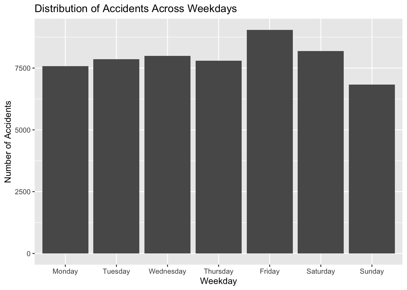
Create the following bar plot showing the distribution of accidents across weekdays.

You can use one of these two methods:

Method 1 : aggregate the dataset with dplyr::count and then use ggplot::geom_bar and the parameter stat = "identity" inside.
Method 2 : do not aggregate the dataset carcteristiques-2022 before plotting.

Solution

# Bar plot for accidents across weekdays

# Method 1
df <- characteristics %>% count(weekday)
weekday_accidents_plot <- 
  ggplot(df) +
  geom_bar(aes(x = weekday, y = n), stat = "identity") +
  labs(x = "Weekday", y = "Number of Accidents",
       title = "Distribution of Accidents Across Weekdays")

# Method 2
weekday_accidents_plot <- 
  ggplot(characteristics) +
  geom_bar(aes(x = weekday)) +
  labs(x = "Weekday", y = "Number of Accidents",
       title = "Distribution of Accidents Across Weekdays")

weekday_accidents_plot

The stat = "identity" parameter is used in the geom_bar() function to indicate that the values on the y-axis of the bar plot should be treated as a variable, rather than being automatically summarized by the plotting function. Indeed, by default, it uses the “statistic” transformation, which calculates the count of occurrences of each category. In contrast, when you use stat = "identity", you are explicitly telling ggplot not to calculate any transformation and to use the raw values provided in the y aesthetic.

Question 6

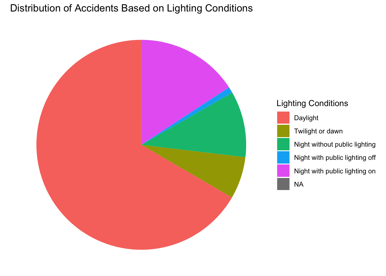
Create a variable lightening_conditions as a factor created using the variable lum. Don’t forget to look at the Variable Dictionary at the end of the document!

To help you to build the factor, you can see the distribution of accidents based on lighting conditions on the following pie chart (you can draw it too as a bonus…).

Solution

# Lightening condition as a factor
characteristics <- characteristics %>% 
  mutate(lightening_conditions = factor(lum, labels= 
                                          c("Daylight",
                                            "Twilight or dawn",
                                            "Night without public lighting",
                                            "Night with public lighting off",
                                            "Night with public lighting on")
                                        ))


# If you want to do the pie chart for lighting conditions
lighting_pie_chart <- ggplot(characteristics) +
  geom_bar(aes(x = "", fill = lightening_conditions),  width = 1) +
  coord_polar("y", start = 0) +
  labs(title = "Distribution of Accidents Based on Lighting Conditions", fill = "Lighting Conditions") +
  theme_void()
lighting_pie_chart

Task 3: Severity Analysis in `usagers-2022.csv`.

Let’s continue with the dataset usagers-2022.csv.

Question 7

Calculate the percentage of accidents that resulted in fatalities (grav == 2).

Solution

Both answers accepted:

Around 2.8% of the accidented people died.

# Percentage of accidents resulting in fatalities
nb_acc <- users %>%
  count()

nb_killed <- 
  users %>%
  filter(grav == 2) %>% 
  count()

100 * nb_killed / nb_acc

         n
1 2.802735

Around 6.0% of the accidents have at least one person who died in it.

# Percentage of accidents resulting in fatalities
nb_acc <- users %>% 
  distinct(Num_Acc) %>% 
  count()

nb_killed <- 
  users %>%
  filter(grav == 2) %>% 
  distinct(Num_Acc) %>% 
  count()


100 * nb_killed / nb_acc

        n
1 6.03414

Question 8

For each dataset (users and characteristics), tell me if you have a different accident ID for each row?

In other words : Is the variable containing the Accident ID a primary key for each dataset? If not, which variable is or could be the primary key?

Solution

In characteristics, the Accident_Id identifier are unique. It is a primary key.

In users, you can find repetition of the Num_Acc variable, because many different users can be involved in the same accident. It is not the primary key.

nrow(characteristics)

[1] 55302

length(unique(characteristics$Accident_Id))

[1] 55302

nrow(characteristics)==length(unique(characteristics$Accident_Id))

[1] TRUE

# Primary key

nrow(users)

[1] 126662

length(unique(users$Num_Acc))

[1] 55302

nrow(users)==length(unique(users$Num_Acc))

[1] FALSE

# Not a primary key

# Any primary key in the dataset ? 
# difficult to understand that code for beginners!
#colnames(users)[which(do.call(c,lapply(colnames(users),function(x){length(unique(users[[x]]))==nrow(users)})))]

nrow(users)

[1] 126662

length(unique(users$id_usager))

[1] 126662

nrow(users)==length(unique(users$id_usager))

[1] TRUE

id_usager is the primary key of the dataset users.

Question 9

Merge the two datasets.

What would be the difference between a full_join and a inner_join here?

Solution

The datasets can be merged using the identifier Num_Acc present in both tables.

# Keep all rows
fullj <- full_join(users, characteristics, by=c("Num_Acc"="Accident_Id"))
nrow(fullj)

[1] 126662

ncol(fullj)

[1] 21

# Keep only commun rows
innerj <- inner_join(users, characteristics,  by=c("Num_Acc"="Accident_Id"))
nrow(innerj)

[1] 126662

ncol(innerj)

[1] 21

Here, both merge do the same thing because the accidents IDs are strictly the same in both datasets.

Submission

Submit a script called exam1_solution.R via email to kim.antunez@sciencespo.fr by the specified deadline : March, 12th before the course of 7:15 pm. Use the email subject: “DSR Exam 1 Submission” and detail the names of the students involved in your group.

Make sure your script is well-organized. It should include clear and concise code, comments explaining your approach, and visualizations (if required).

The answers of the questions must be added in comments using the following syntax:

##############################
## Task 1: Data Preparation ##
##############################

##### Question 1

library(hello)
1+1
# Answer : The average value is 2

Source

The data is obtained on this page.

Variable Dictionary - USAGERS Section

Here is the description of the variables in english. The description in French is in this document

Num_Acc: Accident identifier, identical to the one in the “CARACTERISTIQUES” section, for each user involved in the accident.
id_usager: Unique identifier of the user (including pedestrians attached to vehicles that hit them) - Numeric code.
id_vehicule: Unique identifier of the vehicle for each user occupying it (including pedestrians attached to vehicles that hit them) - Numeric code.
num_Veh: Vehicle identifier for each user occupying it (including pedestrians attached to vehicles that hit them) - Alphanumeric code.
place: Indicates the seat occupied by the user in the vehicle at the time of the accident. Details are given in the document in French.
catu: User category:
- 1 - Driver
- 2 - Passenger
- 3 - Pedestrian
grav: Severity of the user’s injury, classified into three categories of victims plus the unhurt:
- 1 - Unhurt
- 2 - Killed
- 3 - Hospitalized injury
- 4 - Slight injury
sexe: Gender of the user:
- 1 - Male
- 2 - Female
- -1 - Not specified
An_nais: Year of birth of the user.
trajet: Reason for the journey at the time of the accident:
- -1 - Not specified
- 0 - Not specified
- 1 - Home - Work
- 2 - Home - School
- 3 - Errands - Shopping
- 4 - Professional use
- 5 - Leisure - Recreation
- 9 - Other
secu1, secu2, secu3: Safety equipment used by the user until 2018, now indicating usage with up to three possible safety devices for a single user (especially for motorcyclists who are required to wear helmets and gloves).
- -1 - Not specified
- 0 - No equipment
- 1 - Seatbelt
- 2 - Helmet
- 3 - Child device
- 4 - Reflective vest
- 5 - Airbag (2RM/3RM)
- 6 - Gloves (2RM/3RM)
- 7 - Gloves + Airbag (2RM/3RM)
- 8 - Not determinable
- 9 - Other
locp: Pedestrian location:
- -1 - Not specified
- 0 - Not applicable
- On road:
  - 1 - A + 50 m from pedestrian crossing
  - 2 - A - 50 m from pedestrian crossing
- On pedestrian crossing:
  - 3 - No light signal
  - 4 - With light signal
- Miscellaneous:
  - 5 - On sidewalk
  - 6 - On shoulder
  - 7 - On refuge or BAU
  - 8 - On counter lane
  - 9 - Unknown
actp: Pedestrian action:
- -1 - Not specified
- Moving:
  - 0 - Not specified or not applicable
  - 1 - In the direction of the striking vehicle
  - 2 - In the opposite direction of the vehicle
- Miscellaneous:
  - 3 - Crossing
  - 4 - Masked
  - 5 - Playing - Running
  - 6 - With animal
  - 9 - Other
- A - Getting in/out of vehicle
- B - Unknown
etatp: This variable specifies whether the injured pedestrian was alone or not:
- -1 - Not specified
- 1 - Alone
- 2 - Accompanied
- 3 - In a group

Variable Dictionary - CARACTERISTIQUES Section

Here is the description of the variables in english. The description in French is in this document

Num_Acc: Accident identification number.
jour: Day of the accident.
mois: Month of the accident.
an: Year of the accident.
hrmn: Hour and minutes of the accident.
lum: Light: Lighting conditions under which the accident occurred:
- 1 - Daylight
- 2 - Twilight or dawn
- 3 - Night without public lighting
- 4 - Night with public lighting off
- 5 - Night with public lighting on
dep: Department: INSEE Code (National Institute of Statistics and Economic Studies) of the department (2A Corse-du-Sud - 2B Haute-Corse).
com: Municipality: The municipality number is a code given by INSEE. The code consists of the INSEE code of the department followed by 3 digits.
agg: Location:
- 1 - Outside urban area
- 2 - Inside urban area
int: Intersection:
- 1 - Outside intersection
- 2 - X intersection
- 3 - T intersection
- 4 - Y intersection
- 5 - Intersection with more than 4 branches
- 6 - Roundabout
- 7 - Square
- 8 - Level crossing
- 9 - Other intersection
atm: Atmospheric conditions:
- -1 - Not specified
- 1 - Normal
- 2 - Light rain
- 3 - Heavy rain
- 4 - Snow - hail
- 5 - Fog - smoke
- 6 - Strong wind - storm
- 7 - Blinding weather
- 8 - Cloudy weather
- 9 - Other
col: Collision type:
- -1 - Not specified
- 1 - Two vehicles - head-on
- 2 - Two vehicles - rear-end
- 3 - Two vehicles - side impact
- 4 - Three or more vehicles - chain reaction
- 5 - Three or more vehicles - multiple collisions
- 6 - Other collision
- 7 - No collision
adr: Postal address: Variable provided for accidents that occurred inside urban areas.
lat: Latitude
Long: Longitude

Task 1: Data Preparation

Task 2: Data Exploration (carcteristiques-2022.csv)

Task 3: Severity Analysis in usagers-2022.csv.

Submission

Source

Variable Dictionary - USAGERS Section

Variable Dictionary - CARACTERISTIQUES Section

Task 2: Data Exploration (`carcteristiques-2022.csv`)

Task 3: Severity Analysis in `usagers-2022.csv`.