setwd("C:/Desktop/DSR/Session 3")Exercise 1: Visualizing the ‘EU Mood’ indicator
Session 4
This is a demo of how to clean up, summarise and visualize a small dataset, using functions from various {tidyverse} packages.
Download datasets on your computer
Put them a subfolder called data in your working directory.
Load data and install useful packages
First, set your working directory:
repository <- "data"d <- readxl::read_excel(paste0(repository, "/eu-mood.xlsx"), sheet = 2)
head(d)# A tibble: 6 × 55
...1 Belgium ...3 Denmark ...5 France ...7 Germany ...9 Ireland ...11
<chr> <chr> <chr> <chr> <chr> <chr> <chr> <chr> <chr> <chr> <chr>
1 <NA> Mood SE Mood SE Mood SE Mood SE Mood SE
2 1973_2 67.289000… 0.95… 51.232… 0.93 61.63… 1.28… 63.738… 0.70… 56.055… 1.06…
3 1974_1 69.988 0.81… 49.381… 0.83… 61.58… 1.26… 60.984… 0.67… 50.087… 1.002
4 1974_2 66.977999… 0.83 47.439 0.81… 60.753 1.27… 58.734… 0.77… 50.381… 0.998
5 1975_1 69.531000… 0.76… 50.588… 0.83… 61.32… 1.274 59.35 0.75… 52.341… 1.03…
6 1975_2 70.450999… 0.78… 51.69 0.88… 61.85… 1.284 60.722… 0.72… 58.188… 1.07
# ℹ 44 more variables: Italy <chr>, ...13 <chr>, Luxembourg <chr>, ...15 <chr>,
# Netherlands <chr>, ...17 <chr>, UK <chr>, ...19 <chr>, Greece <chr>,
# ...21 <chr>, Portugal <chr>, ...23 <chr>, Spain <chr>, ...25 <chr>,
# Finland <chr>, ...27 <chr>, Austria <chr>, ...29 <chr>, Sweden <chr>,
# ...31 <chr>, Bulgarian <chr>, ...33 <chr>, `Czech Rep` <chr>, ...35 <chr>,
# Estonia <chr>, ...37 <chr>, Hungary <chr>, ...39 <chr>, Latvia <chr>,
# ...41 <chr>, Lithuania <chr>, ...43 <chr>, Malta <chr>, ...45 <chr>, …#install.packages("countrycode")
library(countrycode)library(tidyverse) # {dplyr}, {ggplot2}, {readxl}, {stringr}, {tidyr}, etc.Data Cleaning
You can notice that the dataset is not tidy. We will tidy it step by step.
Clue
- For selecting or removing lines, see
dplyr::slice - For renaming columns, see
dplyr::rename
Solution
d <- d %>%
  # remove first row
  slice(-1) %>%
  # rename first column
  rename(year = "...1")
head(d)
# A tibble: 6 × 55
year Belgium ...3 Denmark ...5 France ...7 Germany ...9 Ireland ...11
<chr> <chr> <chr> <chr> <chr> <chr> <chr> <chr> <chr> <chr> <chr>
1 1973_2 67.289000… 0.95… 51.232… 0.93 61.63… 1.28… 63.738… 0.70… 56.055… 1.06…
2 1974_1 69.988 0.81… 49.381… 0.83… 61.58… 1.26… 60.984… 0.67… 50.087… 1.002
3 1974_2 66.977999… 0.83 47.439 0.81… 60.753 1.27… 58.734… 0.77… 50.381… 0.998
4 1975_1 69.531000… 0.76… 50.588… 0.83… 61.32… 1.274 59.35 0.75… 52.341… 1.03…
5 1975_2 70.450999… 0.78… 51.69 0.88… 61.85… 1.284 60.722… 0.72… 58.188… 1.07
6 1976_1 68.277000… 0.95… 50.414… 0.90… 59.77… 1.292 54.030… 0.96 56.21 1.115
# ℹ 44 more variables: Italy <chr>, ...13 <chr>, Luxembourg <chr>, ...15 <chr>,
# Netherlands <chr>, ...17 <chr>, UK <chr>, ...19 <chr>, Greece <chr>,
# ...21 <chr>, Portugal <chr>, ...23 <chr>, Spain <chr>, ...25 <chr>,
# Finland <chr>, ...27 <chr>, Austria <chr>, ...29 <chr>, Sweden <chr>,
# ...31 <chr>, Bulgarian <chr>, ...33 <chr>, `Czech Rep` <chr>, ...35 <chr>,
# Estonia <chr>, ...37 <chr>, Hungary <chr>, ...39 <chr>, Latvia <chr>,
# ...41 <chr>, Lithuania <chr>, ...43 <chr>, Malta <chr>, ...45 <chr>, …We reshape the dataset from wide to long format below:
d <- d %>%
  # reshape from wide to long
  tidyr::pivot_longer(-year, names_to = "country", values_to = "mood")
head(d)
# A tibble: 6 × 3
year country mood
<chr> <chr> <chr>
1 1973_2 Belgium 67.289000000000001
2 1973_2 ...3 0.95199999999999996
3 1973_2 Denmark 51.232999999999997
4 1973_2 ...5 0.93
5 1973_2 France 61.634999999999998
6 1973_2 ...7 1.2869999999999999
Clue
See dplyr::filter and is.na().
Solution
d <- d %>%
 # keep only rows where ...
  filter(
    # `mood` is non-missing
    !is.na(mood)
  )
Clue
See dplyr::mutate and as.numeric.
Solution
d <- d %>%
   mutate(
    mood = as.numeric(mood)
   )
  head(d)
# A tibble: 6 × 3
year country mood
<chr> <chr> <dbl>
1 1973_2 Belgium 67.3
2 1973_2 ...3 0.952
3 1973_2 Denmark 51.2
4 1973_2 ...5 0.93
5 1973_2 France 61.6
6 1973_2 ...7 1.29 Here are some additional tidying we do:
d <- d %>%
  # keep only rows where ...
  filter(
    # `year` starts with a 4-digit number
    str_detect(year, "^\\d{4}"),
    # `country` starts with a character
    str_detect(country, "^\\w")
  ) %>%
  mutate(
    # convert `year` to year + 0.5 if the value marks Semester 2
    year = str_replace(year, "_1", ".0"),
    year = str_replace(year, "_2", ".5"),
    year = as.numeric(year),
    # semesters and decades
    semester = if_else(year == round(year), 1, 2),
    decade = 10 * as.integer(year) %/% 10,
    # fix country name for Bulgaria
    country = if_else(country == "Bulgarian", "Bulgaria", country)
    )
head(d)
# A tibble: 6 × 5
year country mood semester decade
<dbl> <chr> <dbl> <dbl> <dbl>
1 1974. Belgium 67.3 2 1970
2 1974. Denmark 51.2 2 1970
3 1974. France 61.6 2 1970
4 1974. Germany 63.7 2 1970
5 1974. Ireland 56.1 2 1970
6 1974. Italy 72.8 2 1970Summary statistics by decade
Clue
See dplyr::group_by and dplyr::summarise and use them one after each other using the mean and sd functions inside.
Solution
# decade-level summary for all countries
d %>%
  group_by(decade) %>%
  summarise(
    mu_mood = mean(mood),
    sd_mood = sd(mood)
  )
# A tibble: 5 × 3
decade mu_mood sd_mood
<dbl> <dbl> <dbl>
1 1970 58.9 9.12
2 1980 58.9 9.27
3 1990 57.6 8.52
4 2000 59.1 8.26
5 2010 52.6 7.98We also can also decade-level summary by country
# decade-level summary by country
d %>% group_by(country, decade) %>%
  summarise(
    mu_mood = mean(mood),
    sd_mood = sd(mood)
  )
`summarise()` has grouped output by 'country'. You can override using the
`.groups` argument.# A tibble: 90 × 4
# Groups: country [27]
country decade mu_mood sd_mood
<chr> <dbl> <dbl> <dbl>
1 Austria 1990 47.4 3.81
2 Austria 2000 50.2 3.35
3 Austria 2010 44.4 3.26
4 Belgium 1970 68.8 1.61
5 Belgium 1980 67.0 2.97
6 Belgium 1990 57.1 8.17
7 Belgium 2000 60.9 2.29
8 Belgium 2010 54.3 3.51
9 Bulgaria 2000 69.7 2.88
10 Bulgaria 2010 64.9 3.39
# ℹ 80 more rowsVisualization
Look how we get ISO3-C country codes
# get ISO3-C country codes
d <- d %>%
  mutate(country2 = countrycode::countrycode(country, "country.name", "iso3c"))

# equivalent to
# d$country2 <- countrycode::countrycode(d$country, "country.name", "iso3c")
head(d)
# A tibble: 6 × 6
year country mood semester decade country2
<dbl> <chr> <dbl> <dbl> <dbl> <chr>
1 1974. Belgium 67.3 2 1970 BEL
2 1974. Denmark 51.2 2 1970 DNK
3 1974. France 61.6 2 1970 FRA
4 1974. Germany 63.7 2 1970 DEU
5 1974. Ireland 56.1 2 1970 IRL
6 1974. Italy 72.8 2 1970 ITA
Clue
- Look at the
?uniquevalues ofcountry2. - See
?factor. - See
?levels.
Solution
unique(d$country2) [1] "BEL" "DNK" "FRA" "DEU" "IRL" "ITA" "LUX" "NLD" "GBR" "GRC" "PRT" "ESP"
[13] "FIN" "AUT" "SWE" "BGR" "CZE" "EST" "HUN" "LVA" "LTU" "MLT" "POL" "CYP"
[25] "ROU" "SVK" "SVN"str(d$country2) chr [1:1311] "BEL" "DNK" "FRA" "DEU" "IRL" "ITA" "LUX" "NLD" "GBR" "BEL" ...d <- d %>%
mutate(country2 = factor(country2))
str(d$country2) Factor w/ 27 levels "AUT","BEL","BGR",..: 2 7 11 6 15 16 18 21 12 2 ...levels(d$country2) [1] "AUT" "BEL" "BGR" "CYP" "CZE" "DEU" "DNK" "ESP" "EST" "FIN" "FRA" "GBR"
[13] "GRC" "HUN" "IRL" "ITA" "LTU" "LUX" "LVA" "MLT" "NLD" "POL" "PRT" "ROU"
[25] "SVK" "SVN" "SWE"levels(d$country2)[11][1] "FRA"levels(d$country2)[11] <- "FRC"
levels(d$country2)[11][1] "FRC"d %>% filter(country2 == "FRC") %>% head()# A tibble: 6 × 6
year country mood semester decade country2
<dbl> <chr> <dbl> <dbl> <dbl> <fct>
1 1974. France 61.6 2 1970 FRC
2 1974 France 61.6 1 1970 FRC
3 1974. France 60.8 2 1970 FRC
4 1975 France 61.3 1 1970 FRC
5 1976. France 61.9 2 1970 FRC
6 1976 France 59.8 1 1970 FRC Look how we mark EP election years.
# mark EP election years
e <- c(1979, 1984, 1989, 1994, 1999, 2004, 2009, 2014, 2019)
d$ep_election <- dplyr::if_else(d$year %in% e, d$mood, NA_real_)
head(d)
# A tibble: 6 × 7
year country mood semester decade country2 ep_election
<dbl> <chr> <dbl> <dbl> <dbl> <fct> <dbl>
1 1974. Belgium 67.3 2 1970 BEL NA
2 1974. Denmark 51.2 2 1970 DNK NA
3 1974. France 61.6 2 1970 FRC NA
4 1974. Germany 63.7 2 1970 DEU NA
5 1974. Ireland 56.1 2 1970 IRL NA
6 1974. Italy 72.8 2 1970 ITA NA
Clue
See:
ggplot2::geom_lineggplot2::geom_pointggplot2::facet_wrap
Solution
# line plot, faceted by country
g <- ggplot(d, aes(year, mood)) +
  geom_line() +
  geom_point(aes(y = ep_election), color = "steelblue") +
  facet_wrap(~ country2) +
  theme(
    axis.text = element_blank(),
    axis.ticks = element_blank(),
    axis.title = element_blank(),
    panel.grid = element_blank()
  )
g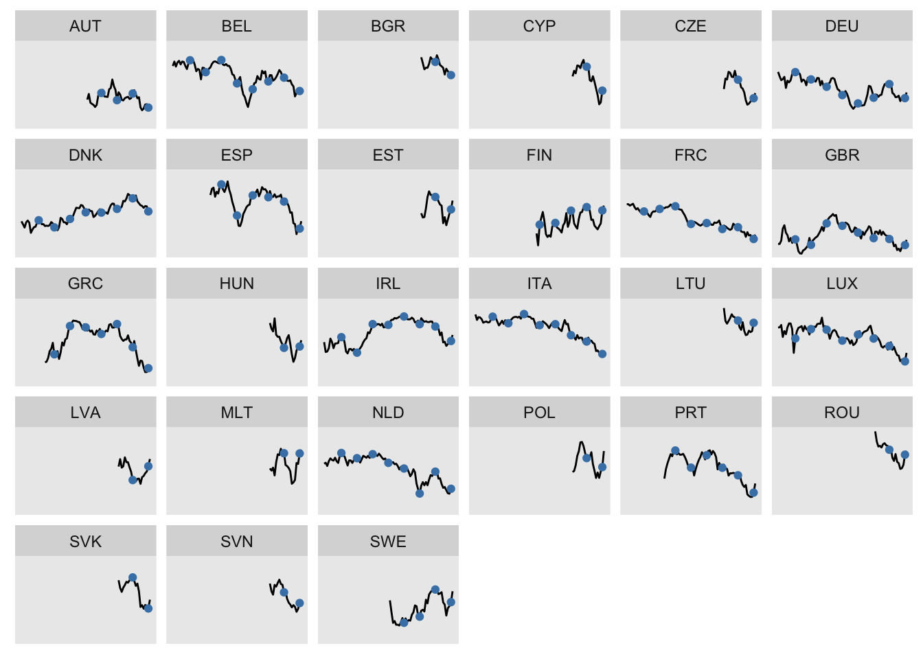
Source
Data sources
Isabelle Guinaudeau and Tinette Schnatterer, “Measuring Public Support for European Integration across Time and Countries: The ‘European Mood’ Indicator,” British Journal of Political Science, 49(3): 1187-1197, 2019.
The dataset comes from the supplementary materials of the article.