library(tidyverse) # {dplyr}, {ggplot2}, {readxl}, {stringr}, {tidyr}, etc.Exercise 2: Economic growth and public debt (Reinhart and Rogoff)
Session 5
Download datasets on your computer
Step 1: Load data and install useful packages
repository <- "data"# read the 'growth' dataset
growth <- readr::read_csv(paste0(repository, "/growth.csv"), show_col_types = FALSE)
glimpse(growth)Rows: 1,275
Columns: 3
$ country <chr> "Australia", "Australia", "Australia", "Australia", "Australia…
$ year <dbl> 1946, 1947, 1948, 1949, 1950, 1951, 1952, 1953, 1954, 1955, 19…
$ growth <dbl> -3.5579515, 2.4594746, 6.4375341, 6.6119938, 6.9202012, 4.2726…# read the 'debt' dataset
debt <- readr::read_csv(paste0(repository, "/debt.csv"), show_col_types = FALSE)
glimpse(debt)Rows: 1,275
Columns: 3
$ country <chr> "Australia", "Australia", "Australia", "Australia", "Australia…
$ year <dbl> 1946, 1947, 1948, 1949, 1950, 1951, 1952, 1953, 1954, 1955, 19…
$ ratio <dbl> 190.41908, 177.32137, 148.92981, 125.82870, 109.80940, 87.0944…# read the 'eu' dataset in tsv and not csv format
eu <- readr::read_tsv(paste0(repository, "/eu-membership.tsv"), show_col_types = FALSE)
glimpse(eu)Rows: 28
Columns: 2
$ country <chr> "Austria", "Belgium", "Bulgaria", "Croatia", "Cyprus", "Czec…
$ accession <dbl> 1995, 1952, 2007, 2013, 2004, 2004, 1973, 2004, 1995, 1952, …Step 2: join them by country-year
Clue
See dplyr::full_join.
Solution
rr <- full_join(growth, debt, by = c("country", "year"))Indeed, note that there are two identifying columns: country and year.
full_join(growth, debt, by = c("country", "year"))# A tibble: 1,275 × 4
country year growth ratio
<chr> <dbl> <dbl> <dbl>
1 Australia 1946 -3.56 190.
2 Australia 1947 2.46 177.
3 Australia 1948 6.44 149.
4 Australia 1949 6.61 126.
5 Australia 1950 6.92 110.
6 Australia 1951 4.27 87.1
7 Australia 1952 0.905 86.1
8 Australia 1953 3.12 79.9
9 Australia 1954 6.22 76.8
10 Australia 1955 5.46 75.0
# ℹ 1,265 more rowsIf you forget the year one, chaos will ensue – you will get two yearcolumns that really should be only one.
full_join(growth, debt, by = "country")Warning in full_join(growth, debt, by = "country"): Detected an unexpected many-to-many relationship between `x` and `y`.
ℹ Row 1 of `x` matches multiple rows in `y`.
ℹ Row 1 of `y` matches multiple rows in `x`.
ℹ If a many-to-many relationship is expected, set `relationship =
"many-to-many"` to silence this warning.# A tibble: 81,305 × 5
country year.x growth year.y ratio
<chr> <dbl> <dbl> <dbl> <dbl>
1 Australia 1946 -3.56 1946 190.
2 Australia 1946 -3.56 1947 177.
3 Australia 1946 -3.56 1948 149.
4 Australia 1946 -3.56 1949 126.
5 Australia 1946 -3.56 1950 110.
6 Australia 1946 -3.56 1951 87.1
7 Australia 1946 -3.56 1952 86.1
8 Australia 1946 -3.56 1953 79.9
9 Australia 1946 -3.56 1954 76.8
10 Australia 1946 -3.56 1955 75.0
# ℹ 81,295 more rowsIf you forget the country one, chaos will ensue – same problem as above, but with countries instead of years
full_join(growth, debt, by = "year")Warning in full_join(growth, debt, by = "year"): Detected an unexpected many-to-many relationship between `x` and `y`.
ℹ Row 1 of `x` matches multiple rows in `y`.
ℹ Row 1 of `y` matches multiple rows in `x`.
ℹ If a many-to-many relationship is expected, set `relationship =
"many-to-many"` to silence this warning.# A tibble: 25,405 × 5
country.x year growth country.y ratio
<chr> <dbl> <dbl> <chr> <dbl>
1 Australia 1946 -3.56 Australia 190.
2 Australia 1946 -3.56 Austria NA
3 Australia 1946 -3.56 Belgium 118.
4 Australia 1946 -3.56 Canada 136.
5 Australia 1946 -3.56 Denmark NA
6 Australia 1946 -3.56 Finland 70.6
7 Australia 1946 -3.56 France NA
8 Australia 1946 -3.56 Germany NA
9 Australia 1946 -3.56 Greece NA
10 Australia 1946 -3.56 Ireland NA
# ℹ 25,395 more rowsStep 3: explore the data
Right now, what you have in your dataset are two time series – here’s the one for debt-to-GDP ratio:
ggplot(rr, aes(x = year, y = ratio, group = country)) +
  geom_line()
Warning: Removed 62 rows containing missing values or values outside the scale range
(`geom_line()`).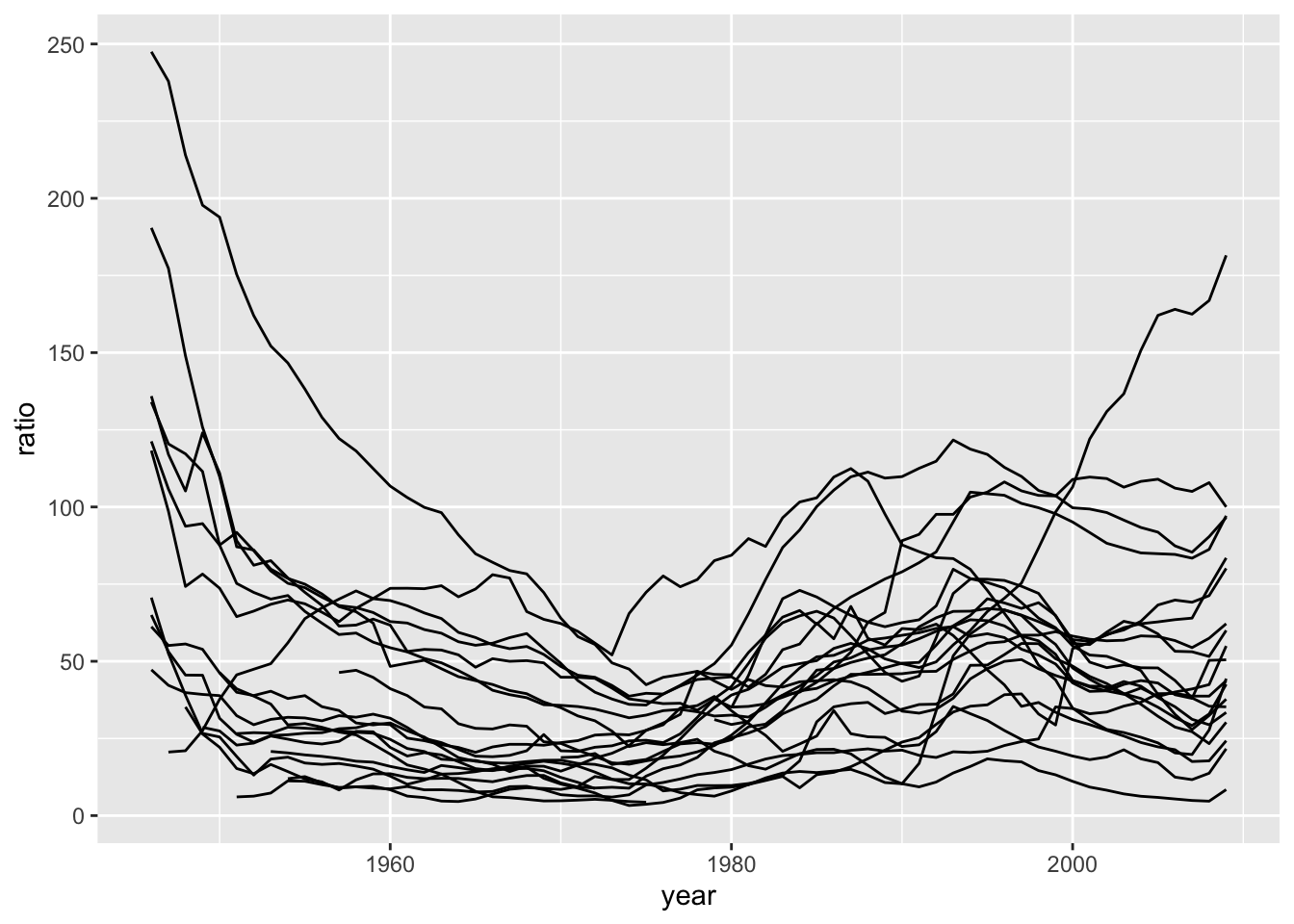
However, the relationship we are interested in is how this ratio relates to the other series, economic growth, so we should be looking at both series together:
ggplot(rr, aes(x = ratio, y = growth)) +
  geom_point()
Warning: Removed 100 rows containing missing values or values outside the scale range
(`geom_point()`).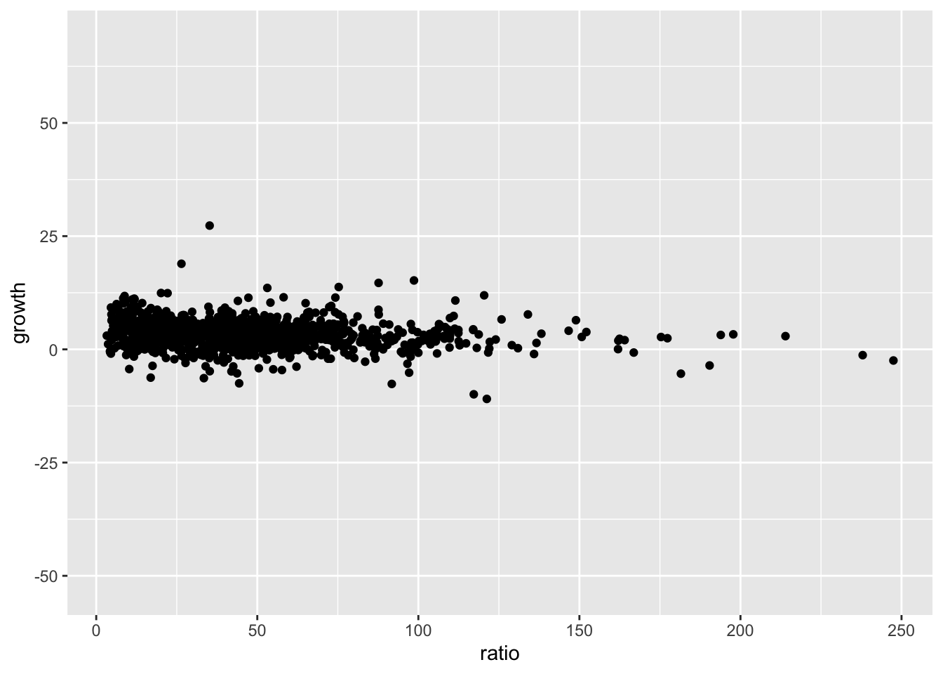
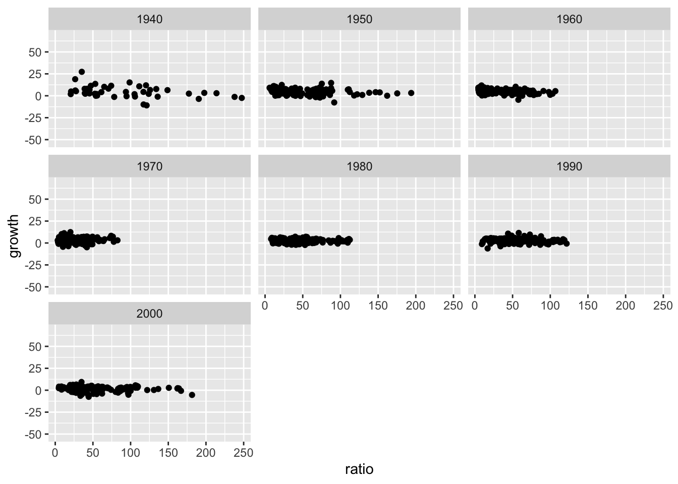
Question 2
Visualizing all data points together is inefficient, so break it down by decade by adding the decade variable to the data and perform this facet graph.
Clue
See:
%/%for a floored integer division (x %/% y := floor(x/y))ggplot2::facet_wrapfor facetting the graph as below
Solution
# add decade
 rr <- rr %>% mutate(decade = 10 * year %/% 10)
# equivalent to:
# rr$decade <- 10 * rr$year %/% 10

# this allows to break down the plot into small multiples (facets)
ggplot(rr, aes(x = ratio, y = growth, group = country)) +
  geom_point() +
  facet_wrap(~ decade)
We’re getting somewhere, but if you inspect the data, you will find missing values – which can be excluded by using the tidyr::drop_na function, which will exclude all rows that hold any missing values (more on that later).
ggplot( tidyr::drop_na(rr), aes(x = ratio, y = growth, group = country)) +
  geom_point() +
  facet_wrap(~ decade)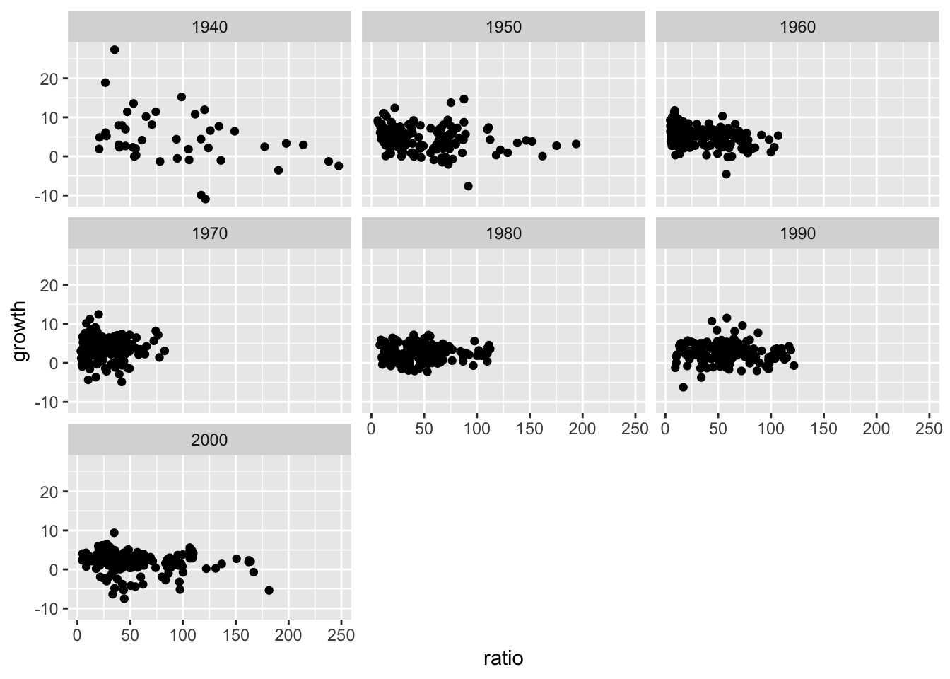
Let’s reformulate the two steps above (creating decades and excluding rows with missing values) into a ‘chain’ of functions that does the same thing:
rr <- rr %>%
  mutate(decade = 10 * year %/% 10) %>%
  tidyr::drop_na(growth, ratio)

# Last line is equivalent to
# dplyr::filter(!is.na(growth) & !is.na(ratio))
The reformulation is syntactically more compact, and also more careful than what we did earlier, as we specify which variables should be used by the drop_na function to remove missing values: this makes sure that no other variable present in the dataset gets accidentally taken into account at that step, which could have led to excessive data loss.
Another way to write that step safely is to use filter(!is.na(growth), !is.na(ratio)).
Step 4: highlight EU member states
We’re getting where we want to be…
ggplot(rr, aes(ratio, growth)) +
  geom_point(color = "grey50", alpha = 3/4) +
  geom_smooth(color = "black", se = FALSE) +
  facet_wrap(~ decade, nrow = 1, scales = "free_x")
`geom_smooth()` using method = 'loess' and formula = 'y ~ x'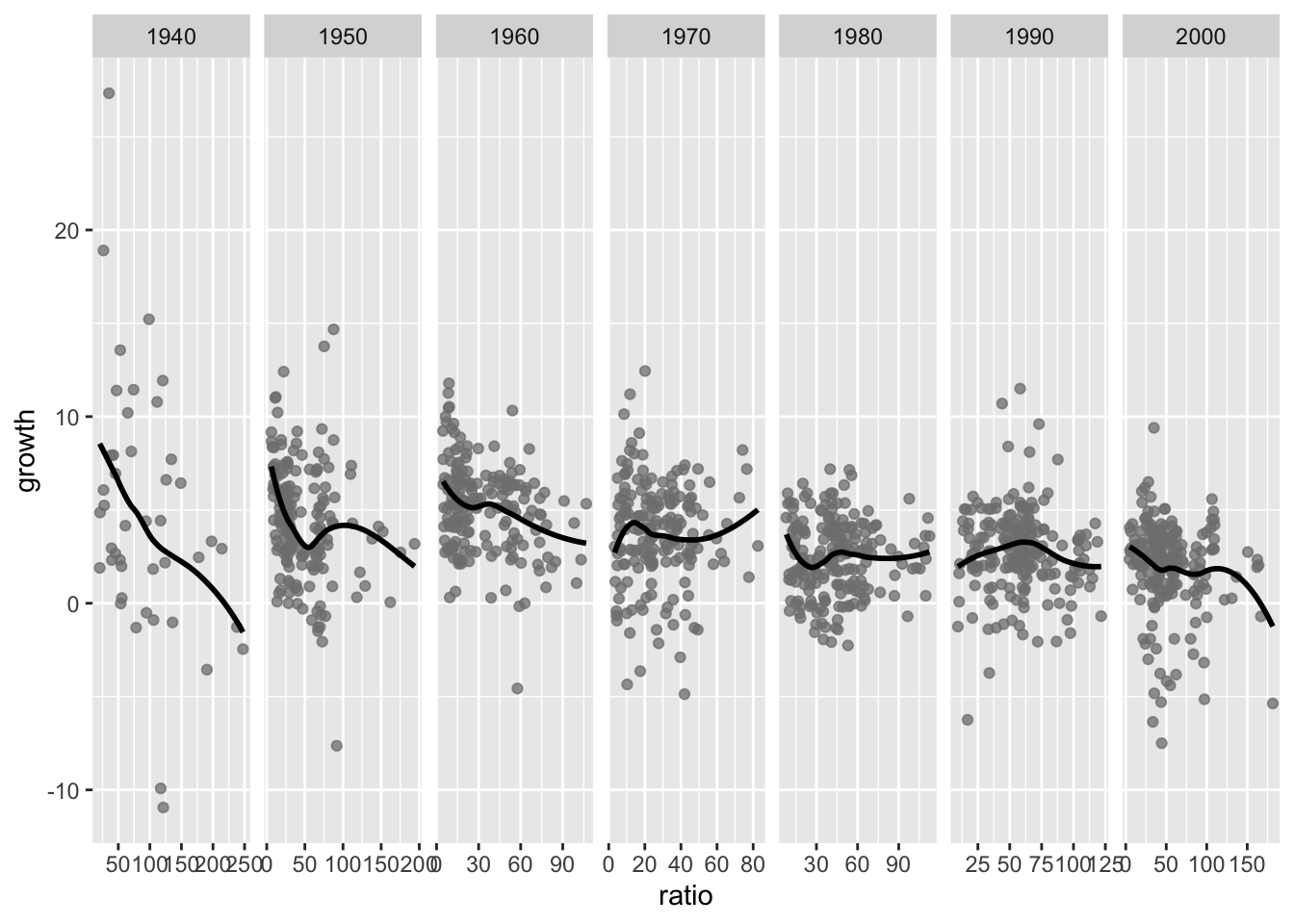
Clue
See dplyr::left_join.
Solution
rr <- left_join(rr, eu, by = "country")See the results for e.g. Belgium:
rr %>%
  filter(country == "Belgium")
# A tibble: 63 × 6
country year growth ratio decade accession
<chr> <dbl> <dbl> <dbl> <dbl> <dbl>
1 Belgium 1947 15.2 98.6 1940 1952
2 Belgium 1948 11.4 74.2 1940 1952
3 Belgium 1949 -1.31 78.3 1940 1952
4 Belgium 1950 5.64 73.7 1950 1952
5 Belgium 1951 7.03 64.5 1950 1952
6 Belgium 1952 -0.430 66.3 1950 1952
7 Belgium 1953 2.93 68.5 1950 1952
8 Belgium 1954 -1.27 69.9 1950 1952
9 Belgium 1955 5.15 68.6 1950 1952
10 Belgium 1956 2.43 65.9 1950 1952
# ℹ 53 more rowsSince EU membership has a start date (accession), let’s create a variable to identify the rows where the country has joined the EU.
rr <-  rr %>%
  mutate(
    # mark EU membership as TRUE or FALSE
    joined_eu = !is.na(accession) & year >= accession,
    # replace `TRUE` with "EU", `FALSE` with "Non-EU"
    joined_eu = if_else(joined_eu, "EU", "Non-EU")
  )
Step 5: highlight EU member states
Here is the plot with EU member states highlighted
ggplot(rr, aes(ratio, growth)) +
  geom_point(aes(color = joined_eu), alpha = 3/4) +
  geom_smooth(color = "black", se = FALSE) +
  facet_wrap(~ decade, nrow = 1, scales = "free_x") +
  scale_color_manual("", values = c("EU" = "steelblue", "Non-EU" = "grey50")) +
  theme_linedraw() +
  labs(y = "GDP growth (%)", x = "debt-to-GDP ratio")
`geom_smooth()` using method = 'loess' and formula = 'y ~ x'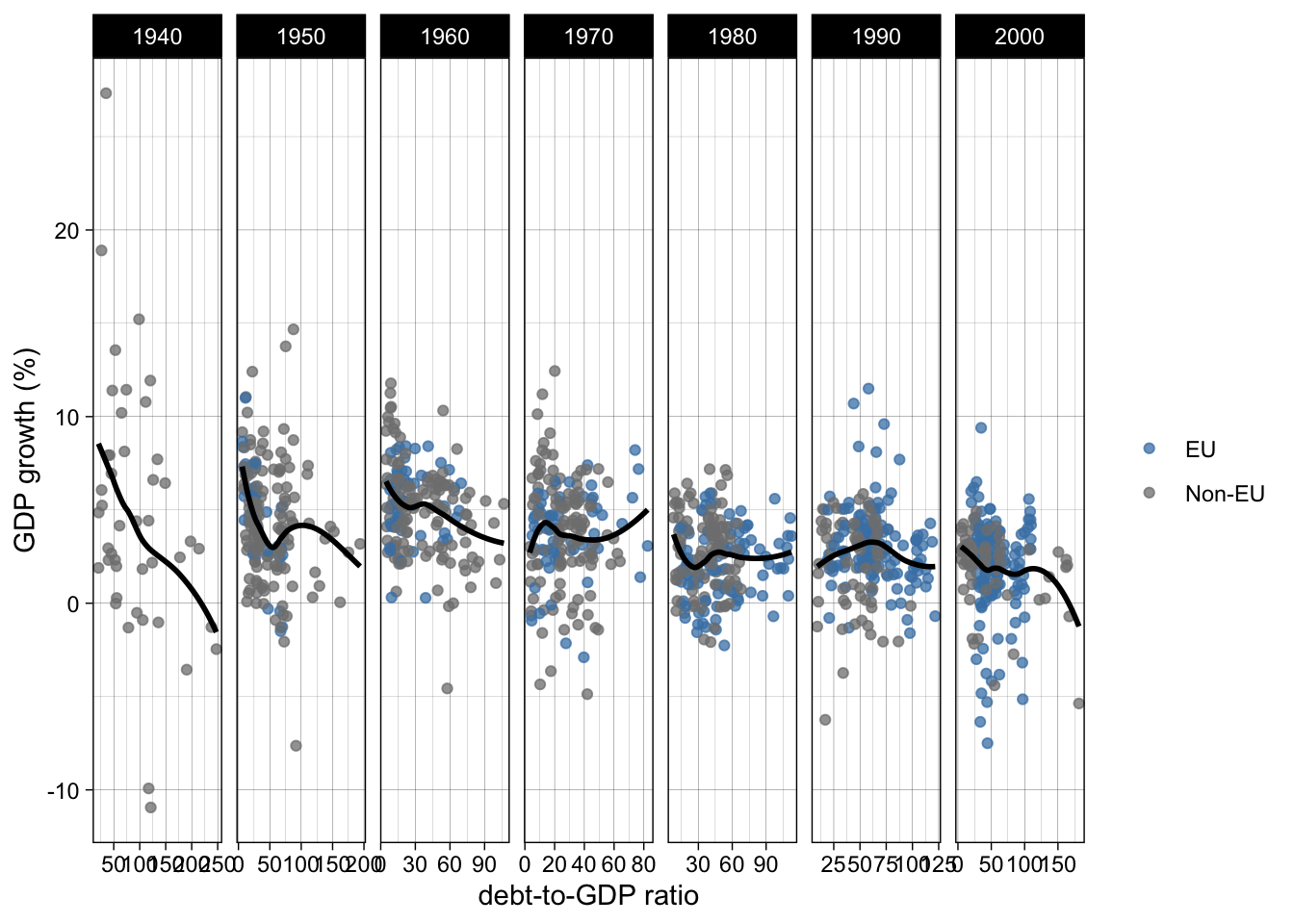
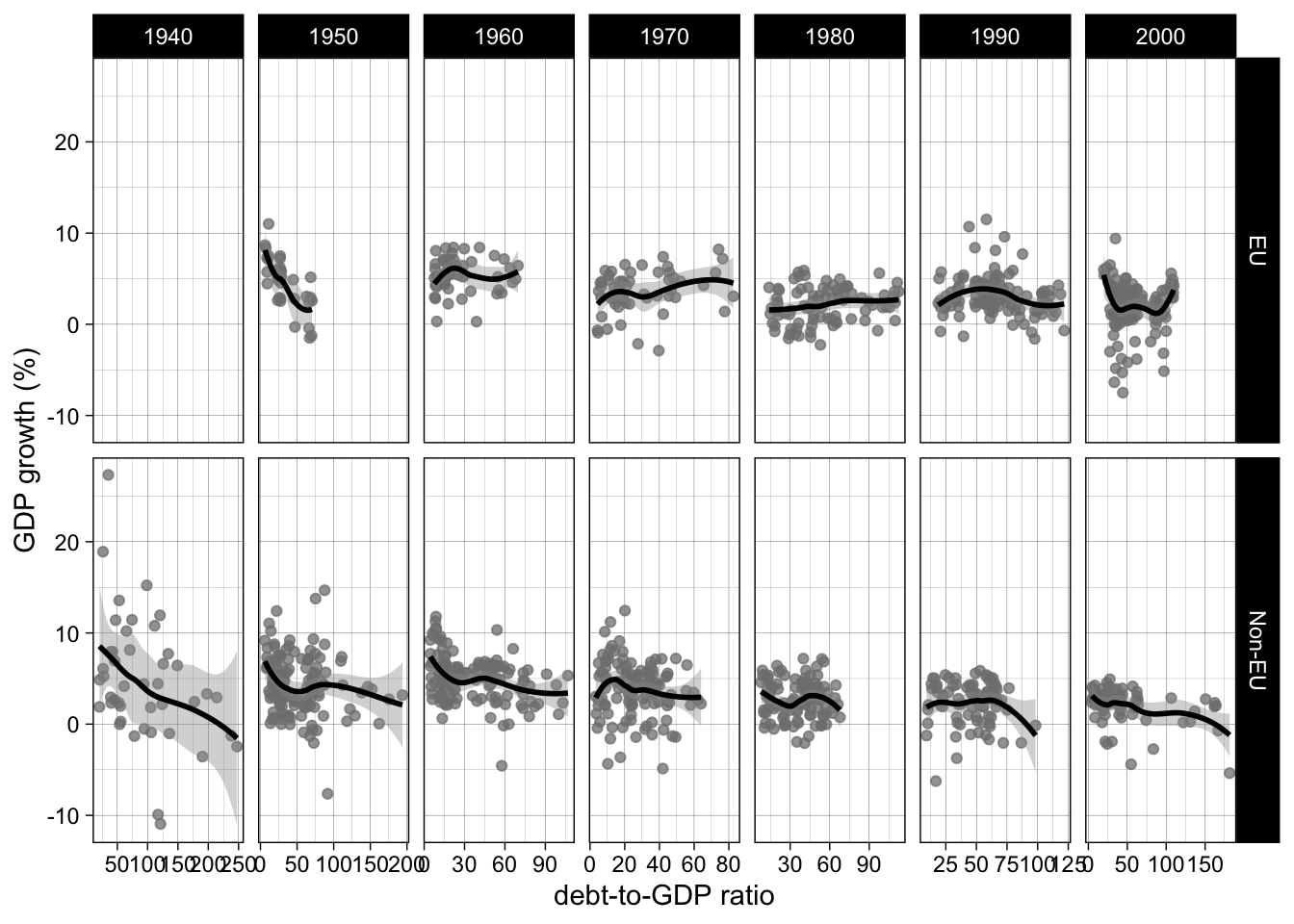
Question 4
Try to perform this plot, with a variation that splits the data by EU membership.
Clue
- See
ggplot2::geom_smoothand theseparameter equals toTRUE - Use
ggplot2::facet_gridinstead ofggplot2::facet_wrapand use in additing the variablejoined_eu
Solution
ggplot(rr, aes(ratio, growth)) +
  geom_point(color = "grey50", alpha = 3/4) +
  geom_smooth(color = "black", se = TRUE) +
  facet_grid(joined_eu ~ decade, scales = "free_x") +
  theme_linedraw() +
  labs(y = "GDP growth (%)", x = "debt-to-GDP ratio")
Source
Data sources
Thomas Herndon, Michael Ash and Robert Pollin, “Does high public debt consistently stifle economic growth? A critique of Reinhart and Rogoff,” Cambridge Journal of Economics 38(2): 257–79, 2014.
The data come from the Zenodo repository of the study. You can read the backstory of this example on Andrew Gelman’s blog.
R code to generate the debt and growth datasets
Using the previously mentioned replication package by Herndon et al.:
library(tidyverse)

fs::dir_create("data")

rr <- "WP322HAP-RR-GITD-code-2013-05-17/RR-processed.dta" %>%
  haven::read_dta() %>%
  select(country = Country, year = Year, growth = dRGDP, ratio = debtgdp) %>%
  mutate(country = as.character(haven::as_factor(country)))

readr::write_csv(select(rr, -growth), "data/debt.csv")
readr::write_csv(select(rr, -ratio), "data/growth.csv")
R code to generate the eu-membership dataset
Using Wikipedia, for lack of a better source, since the EU Commission does not seem to have it anywhere on its website:
library(countrycode)
library(rvest)
library(tidyverse)

h <- "https://en.wikipedia.org/wiki/Enlargement_of_the_European_Union" %>%
  rvest::read_html()

rvest::html_table(h) %>%
  pluck(3) %>%
  select(country = Applicant, accession = `Accession / failure rationale`) %>%
  filter(!str_detect(accession, "Frozen|Negotiating|Rejected|Withdrawn")) %>%
  filter(!str_detect(accession, "Applicant|Candidate|Vetoed")) %>%
  mutate(
    country = countrycode::countrycode(country, "country.name", "country.name"),
    accession = as.integer(str_extract(accession, "\\d{4}"))
  ) %>%
  readr::write_tsv("data/eu-membership.tsv")