library(tidyverse) # {dplyr}, {ggplot2}, {readxl}, {stringr}, {tidyr}, etc.Exercise 1: Colonialism, democracy, life expectancy and wealth [Part 1]
Session 6
This is an example inspired by research into the historical legacy of colonialism, using the Quality of Government cross-sectional dataset.
N.B. This exercise also includes some more advanced data manipulation code that illustrates:
- how to handle labelled variables imported from Stata or SPSS
- how to create factor variables.
You might need to read from your handbooks to make sure that you understand how factor variables work.
Download datasets on your computer
Load data and install useful packages
repository <- "data"library(haven) # functions for working with Stata datasets
library(MASS) # functions for fitting distributions
Attaching package: 'MASS'The following object is masked from 'package:dplyr':
selectlibrary(moments) # functions for skewness and kurtosis
# library(e1071) # more functions for skewness and kurtosis (optional)d <- haven::read_dta(paste0(repository, "/qog_std_cs_jan23_stata14.dta"))glimpse(d)str(d)
head(d)About the dataset
nrow(d) [1] 194ncol(d) [1] 1705This is a very large dataset, but it comes with excellent documentation: make sure to refer to the codebook when relevant.
Also note that thanks to the dataset having been imported in Stata format, some of its variables have labels, as is the case for colonial origin:
table(d$ht_colonial)
 0  1  2  3  4  5  6  7  8  9 10
71  2 19  2  4 58 26  6  3  1  2
The variable is numerically encoded, but the values carry labels for ease of use when coding; values are also listed in the codebook, with more details
haven::print_labels(d$ht_colonial)
Labels:
 value                                                   label
     0 0. Never colonized by a Western overseas colonial power
     1                                                1. Dutch
     2                                              2. Spanish
     3                                              3. Italian
     4                                                   4. US
     5                                              5. British
     6                                               6. French
     7                                           7. Portuguese
     8                                              8. Belgian
     9                                       9. British-French
    10                                          10. Australian
The easiest way to access those labels is to convert the variable into a factor variable, which is a variable type that you should have read about in your handbooks:
head(haven::as_factor(d$ht_colonial), 9) # first 9 observations/values[1] 0. Never colonized by a Western overseas colonial power
[2] 0. Never colonized by a Western overseas colonial power
[3] 6. French
[4] 0. Never colonized by a Western overseas colonial power
[5] 7. Portuguese
[6] 5. British
[7] 0. Never colonized by a Western overseas colonial power
[8] 2. Spanish
[9] 0. Never colonized by a Western overseas colonial power
11 Levels: 0. Never colonized by a Western overseas colonial power ... 10. Australianlevels(haven::as_factor(d$ht_colonial)) # levels of the factor variable [1] "0. Never colonized by a Western overseas colonial power"
[2] "1. Dutch"
[3] "2. Spanish"
[4] "3. Italian"
[5] "4. US"
[6] "5. British"
[7] "6. French"
[8] "7. Portuguese"
[9] "8. Belgian"
[10] "9. British-French"
[11] "10. Australian" Describe a numerical variable (life expectancy)
Clue
Remember the is.na() function. And in R, does not respect this condition is written !condition.
Solution
# Summary
summary(d$wdi_lifexp)
Min. 1st Qu. Median Mean 3rd Qu. Max. NA's
52.91 66.60 73.18 72.33 77.90 84.36 9 # Missing values?
sum(is.na(d$wdi_lifexp)) # number of missing values[1] 9sum(!is.na(d$wdi_lifexp)) # number of nonmissing observations[1] 185Indeed, the missing values will force us to use na.rm = TRUE in other functions to obtain summary statistics, such as the functions to obtain quantiles:
median(d$wdi_lifexp, na.rm = TRUE)[1] 73.18quantile(d$wdi_lifexp, na.rm = TRUE) 0% 25% 50% 75% 100%
52.91000 66.60300 73.18000 77.90488 84.35634 Without that argument, missing values will propagate and the result of those functions will itself be a missing value
median(d$wdi_lifexp)[1] NAHere are the other measures of dispersion
range(d$wdi_lifexp, na.rm = TRUE)[1] 52.91000 84.35634var(d$wdi_lifexp, na.rm = TRUE)[1] 56.88383sd(d$wdi_lifexp, na.rm = TRUE)[1] 7.542137Here are some useful plots
# histogram
ggplot(d, aes(x = wdi_lifexp)) +
  geom_histogram(bins = 10, color = "white")
Warning: Removed 9 rows containing non-finite outside the scale range
(`stat_bin()`).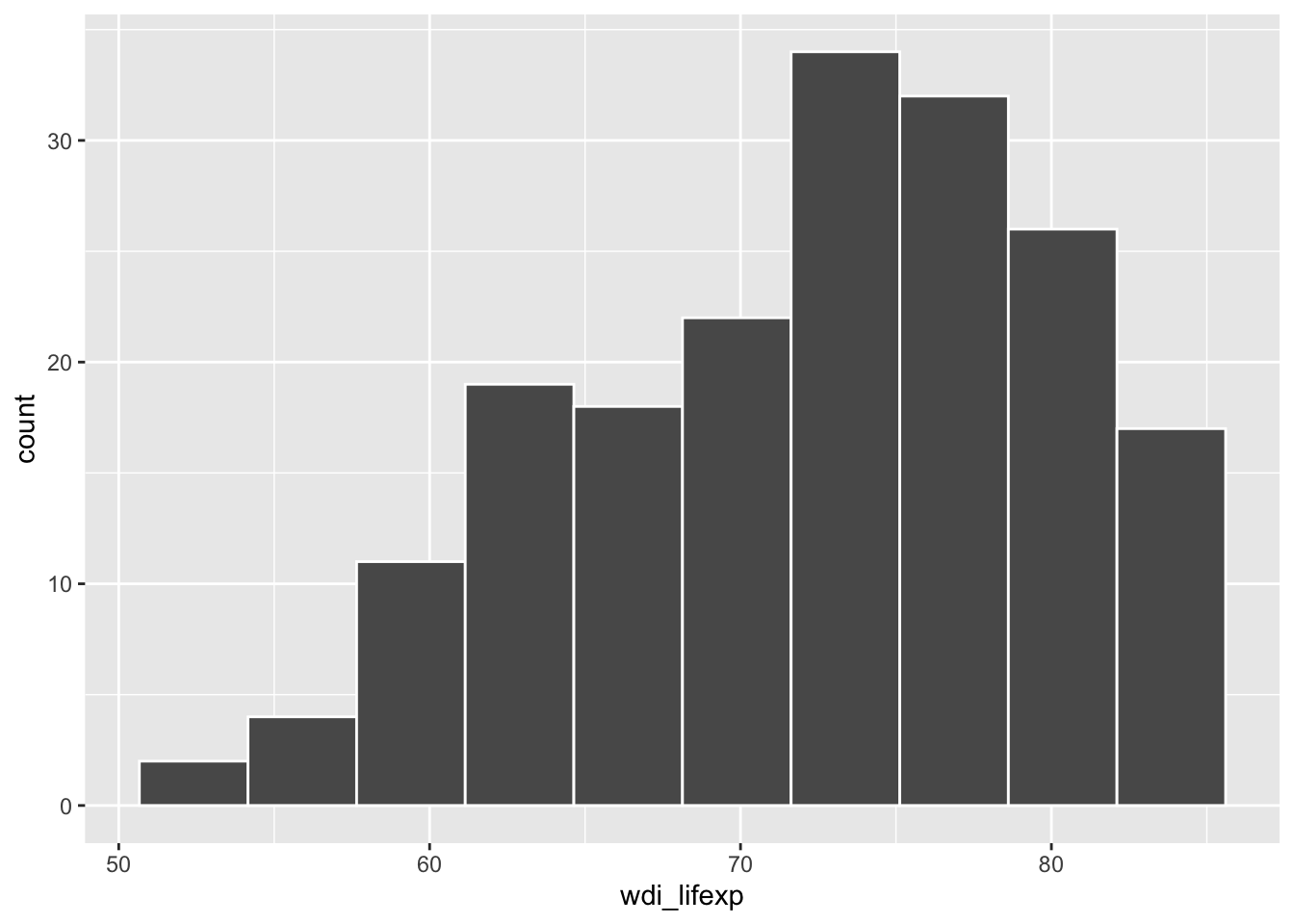
# density curve
ggplot(d, aes(x = wdi_lifexp)) +
  geom_density()
Warning: Removed 9 rows containing non-finite outside the scale range
(`stat_density()`).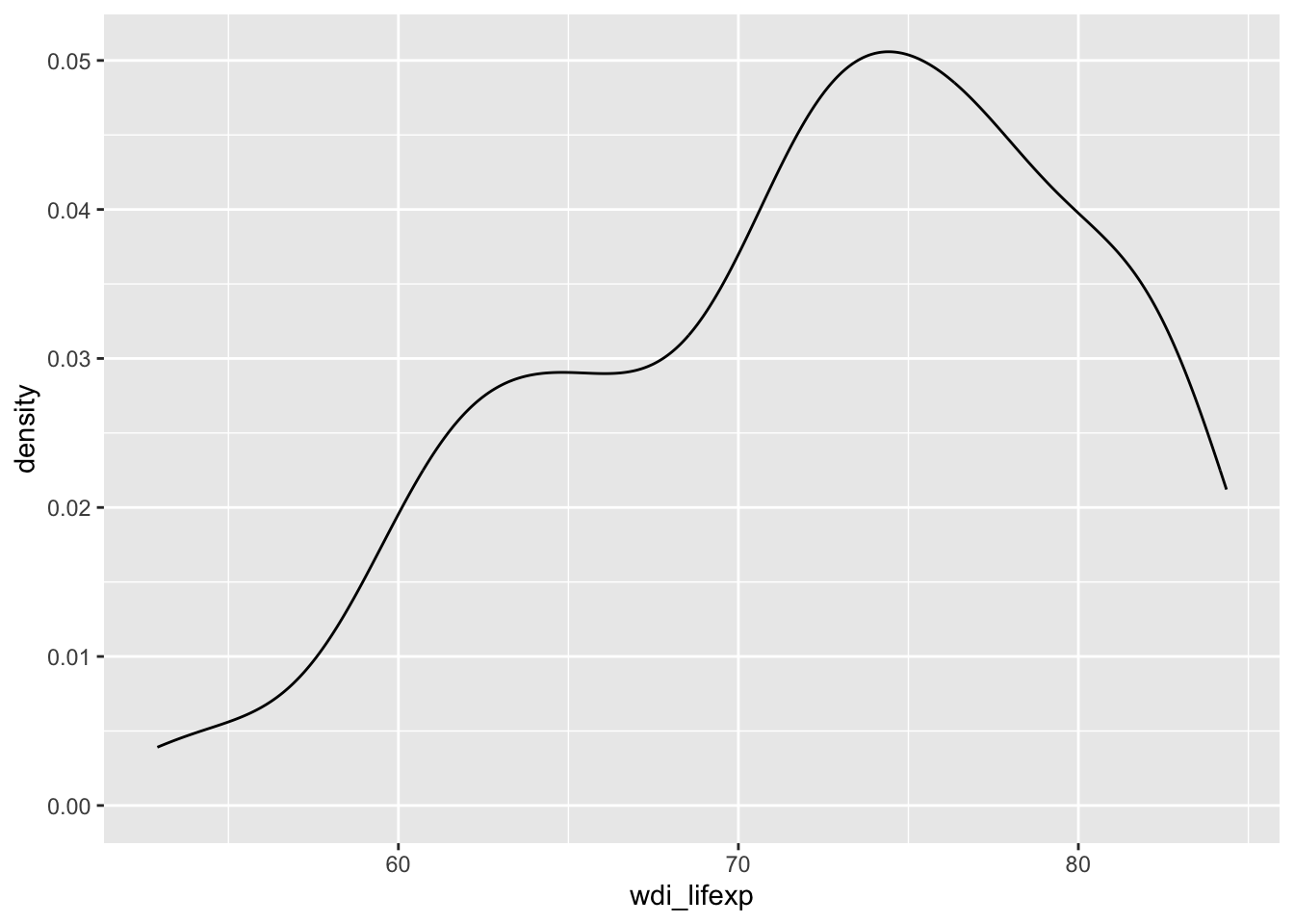
# cumulative distribution
ggplot(d, aes(y = wdi_lifexp)) +
  geom_step(stat = "ecdf") + # empirical cumulative distribution function
  labs(x = "percentile")
Warning: Removed 9 rows containing non-finite outside the scale range
(`stat_ecdf()`).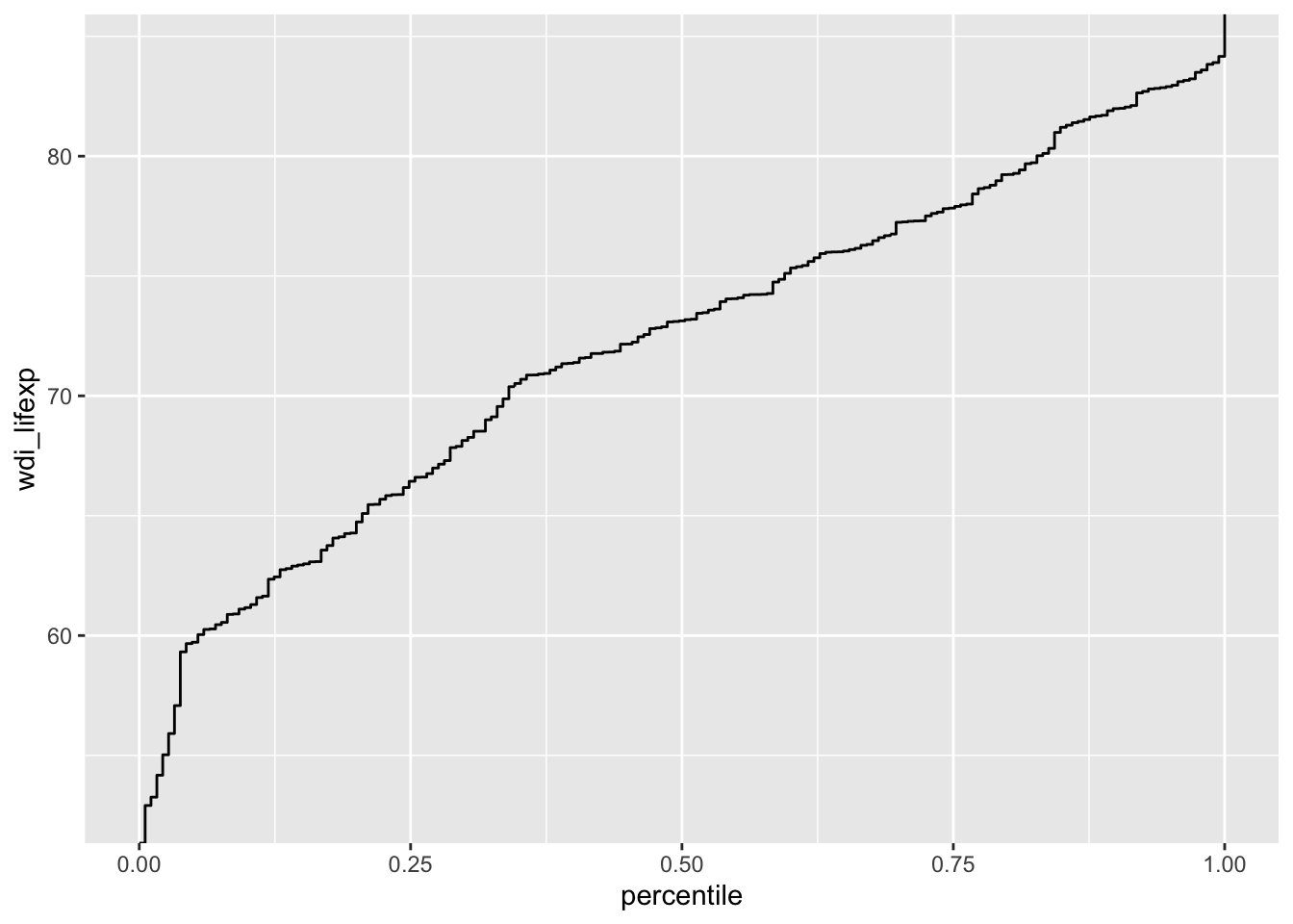
Describe a categorical (dummy) variable
Variable 1: Colonial origin
To summarise a categorical variable and check for missing values:
table(d$ht_colonial, exclude = NULL)
 0  1  2  3  4  5  6  7  8  9 10
71  2 19  2  4 58 26  6  3  1  2
Here there is no missing values.
Show the value labels and their counts (i.e. raw/absolute frequencies)
d %>% count(haven::as_factor(ht_colonial))# A tibble: 11 × 2
`haven::as_factor(ht_colonial)` n
<fct> <int>
1 0. Never colonized by a Western overseas colonial power 71
2 1. Dutch 2
3 2. Spanish 19
4 3. Italian 2
5 4. US 4
6 5. British 58
7 6. French 26
8 7. Portuguese 6
9 8. Belgian 3
10 9. British-French 1
11 10. Australian 2Add percentages (i.e. relative frequencies)
d %>%
  count(haven::as_factor(ht_colonial)) %>%
  mutate(percent = 100 * n / sum(n))
# A tibble: 11 × 3
`haven::as_factor(ht_colonial)` n percent
<fct> <int> <dbl>
1 0. Never colonized by a Western overseas colonial power 71 36.6
2 1. Dutch 2 1.03
3 2. Spanish 19 9.79
4 3. Italian 2 1.03
5 4. US 4 2.06
6 5. British 58 29.9
7 6. French 26 13.4
8 7. Portuguese 6 3.09
9 8. Belgian 3 1.55
10 9. British-French 1 0.515
11 10. Australian 2 1.03 Let’s recode the variable as a dummy through various methods
d$former_colony1 <- d$ht_colonial != 0
table(d$former_colony1, exclude = NULL) # logical
FALSE  TRUE
71 123 d$former_colony2 <- as.integer(d$ht_colonial != 0)
table(d$former_colony2, exclude = NULL) # integer (numeric)
  0   1
71 123 d$former_colony3 <- if_else(d$ht_colonial == 0, "No", "Yes")
table(d$former_colony3, exclude = NULL) # character
 No Yes
 71 123
Percentage of formerly colonized countries
prop.table(table(d$former_colony1, exclude = NULL))
    FALSE      TRUE
0.3659794 0.6340206
… or better, using dplyr::count as shown earlier
d %>%
  count(former_colony1) %>%
  mutate(percent = 100 * n / sum(n))
# A tibble: 2 × 3
former_colony1 n percent
<lgl> <int> <dbl>
1 FALSE 71 36.6
2 TRUE 123 63.4Next, a (lowly informative) bar plot of the frequencies of that variable
ggplot(d, aes(x = former_colony1)) +
  geom_bar()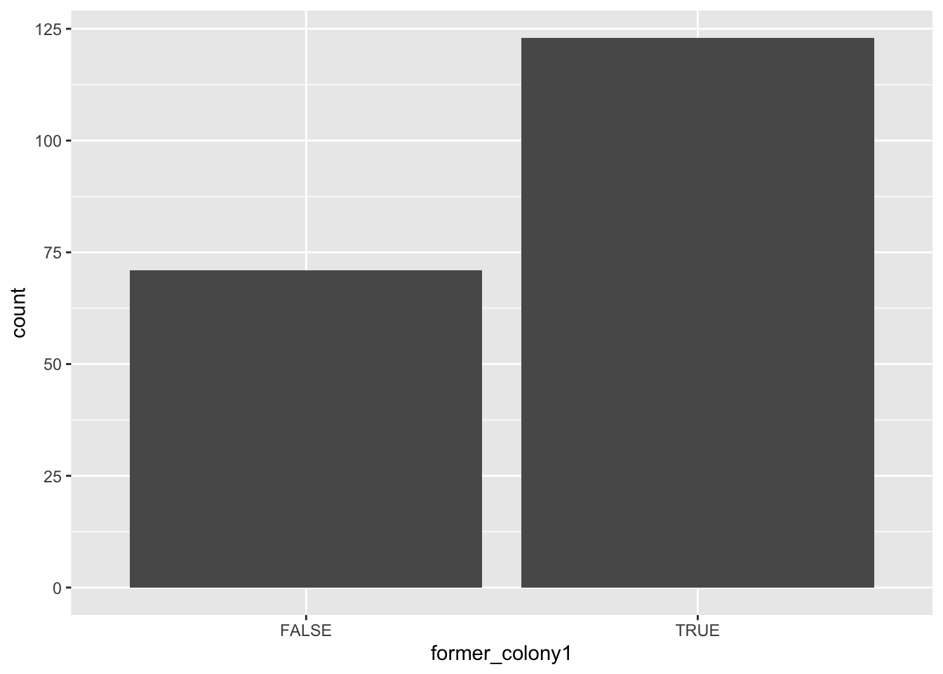
… or better, percentages, using dplyr::count as shown earlier
d %>%
  count(former_colony1) %>%
  mutate(percent = 100 * n / sum(n)) %>%
  ggplot(aes(x = former_colony1, y = percent)) +
  geom_bar(stat = "identity")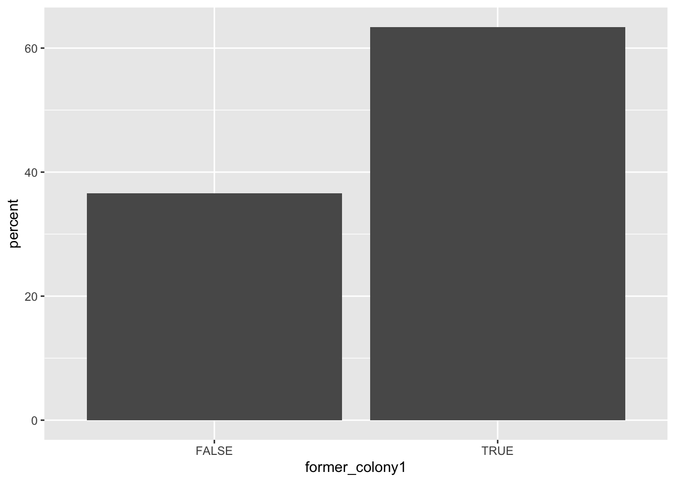
And last, another example of creating a factor variable.
Again, refer to your handbook readings to make sure that you understand how to handle factors, as they will be useful at later stages of analysis
d$former_colony <- factor(d$ht_colonial != 0)
str(d$former_colony)
Factor w/ 2 levels "FALSE","TRUE": 1 1 2 1 2 2 1 2 1 1 ...levels(d$former_colony)[1] "FALSE" "TRUE" levels(d$former_colony) <- c("Never colonized", "Former colony")
# Or : d$former_colony <- factor(d$ht_colonial, labels = c("Never colonized", "Former colony"))Final result:
table(d$former_colony, exclude = NULL)
Never colonized   Former colony
             71             123
Or as percentages, using base R
round(100 * prop.table(table(d$former_colony)), 2)
Never colonized   Former colony
           36.6            63.4
Variable 2: Regime type
Solution
table(d$br_dem, exclude = NULL)
   0    1 <NA>
  74  118    2
Here there is 2 NA in the dataset!
d %>% count(haven::as_factor(br_dem))# A tibble: 3 × 2
`haven::as_factor(br_dem)` n
<fct> <int>
1 0 74
2 1 118
3 <NA> 2d %>%
count(haven::as_factor(br_dem)) %>%
mutate(percent = 100 * n / sum(n))# A tibble: 3 × 3
`haven::as_factor(br_dem)` n percent
<fct> <int> <dbl>
1 0 74 38.1
2 1 118 60.8
3 <NA> 2 1.03d$democratic <- factor(d$br_dem, labels = c("Nondemocratic", "Democratic"))
str(d$democratic) Factor w/ 2 levels "Nondemocratic",..: 1 2 1 NA 1 2 1 2 2 2 ...levels(d$democratic)[1] "Nondemocratic" "Democratic" prop.table(table(d$democratic, exclude = NULL))
Nondemocratic    Democratic          <NA>
0.38144330 0.60824742 0.01030928 prop.table(table(d$democratic))
Nondemocratic    Democratic
    0.3854167     0.6145833
d %>%
count(democratic) %>%
mutate(percent = 100 * n / sum(n))# A tibble: 3 × 3
democratic n percent
<fct> <int> <dbl>
1 Nondemocratic 74 38.1
2 Democratic 118 60.8
3 <NA> 2 1.03d %>%
count(democratic) %>%
mutate(percent = 100 * n / sum(n)) %>%
ggplot(aes(x = democratic, y = percent)) +
geom_bar(stat = "identity")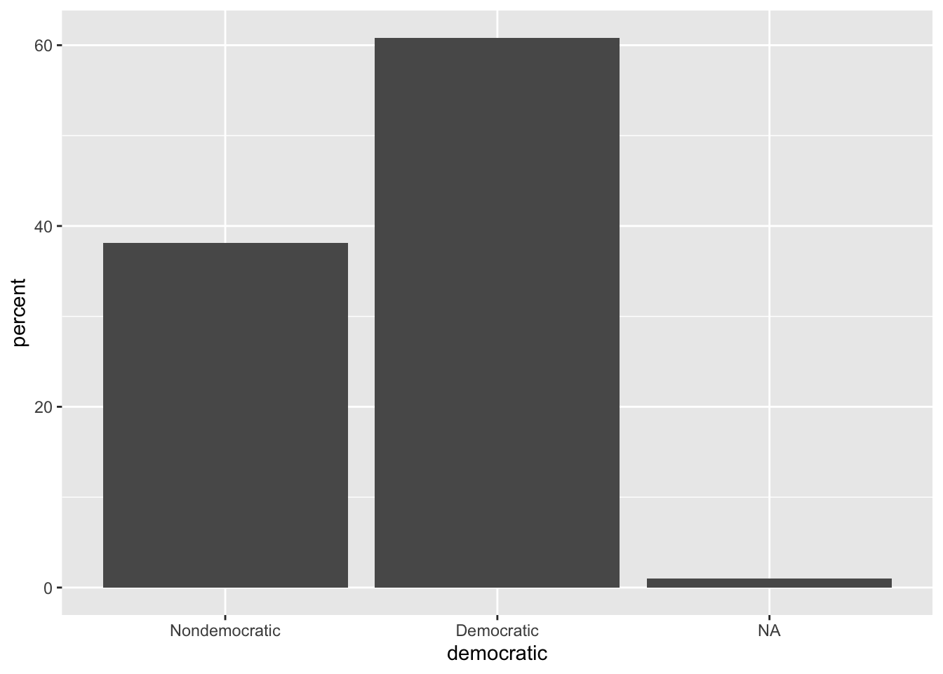
Normality assessment and logarithmic transformations [OPTIONAL]
# distribution of GDP/capita
ggplot(d, aes(x = wdi_gdpcappppcur)) +
  geom_density() #+
Warning: Removed 11 rows containing non-finite outside the scale range
(`stat_density()`).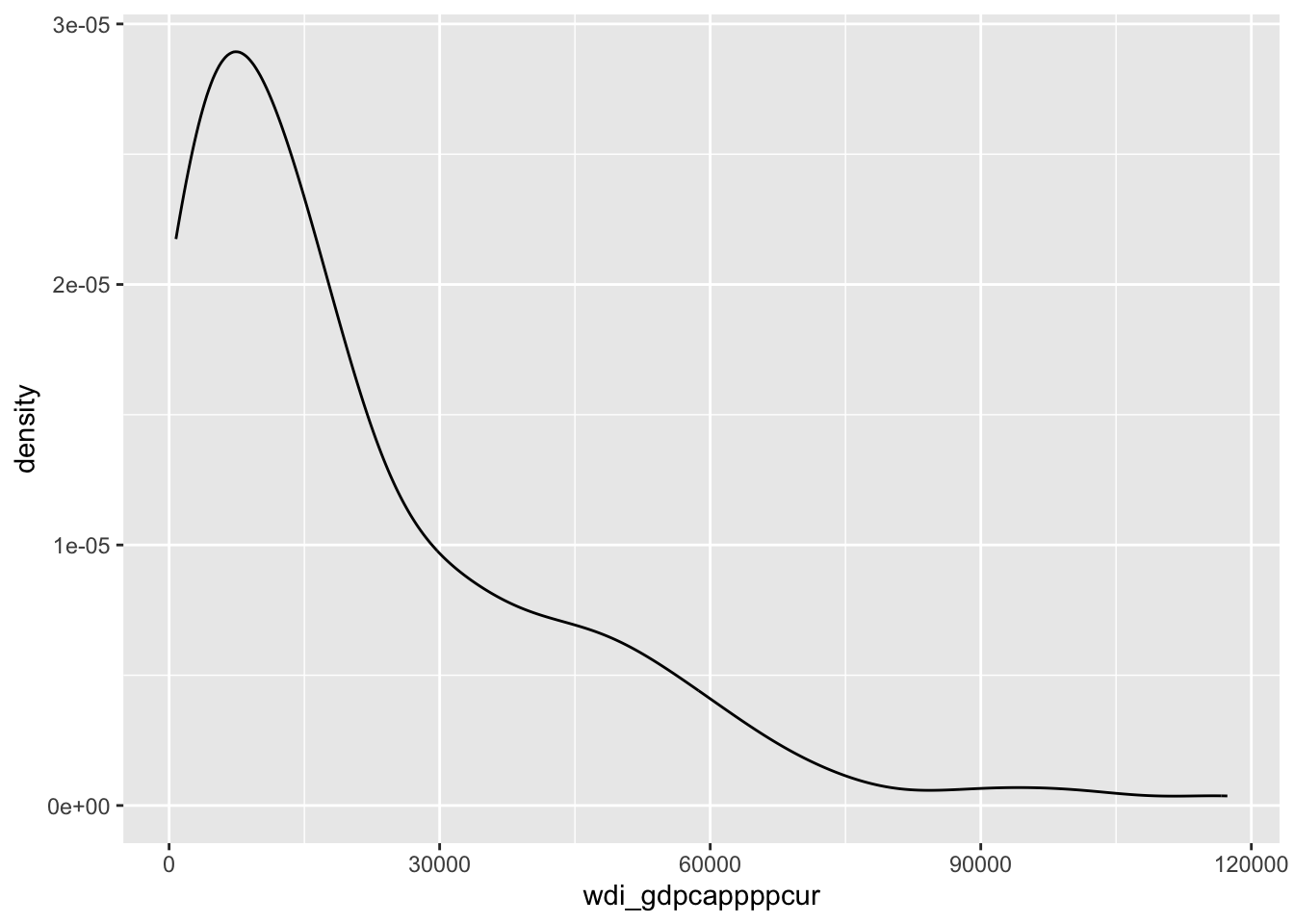
#geom_rug()This variable is very unevenly distributed, with many outliers, which are easier to spot when the data are broken down by geographic region:
ggplot(d, aes(x = wdi_gdpcappppcur)) +
  geom_boxplot(aes(y = haven::as_factor(ht_region)))
Warning: Removed 11 rows containing non-finite outside the scale range
(`stat_boxplot()`).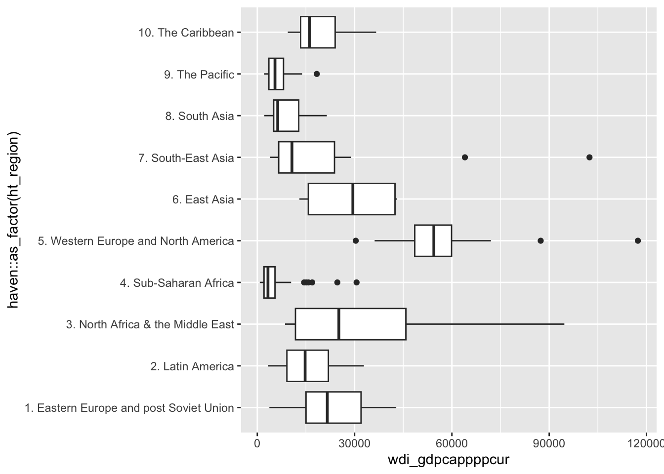
Normality assessment:
moments::skewness(d$wdi_gdpcappppcur, na.rm = TRUE) #0 for normal distribution[1] 1.62173moments::kurtosis(d$wdi_gdpcappppcur, na.rm = TRUE) #~3 for normal distribution[1] 5.912613Note that there are multiple ways of computing the statistics above, as shown by the functions of the {e1071} functions package, which each provide three different methods.
At that stage, it makes sense to look for a transformation of the unit of measurement of the variable, in order to better approach normality; the most obvious candidate is often logarithmic units:
d$log_gdpc <- log(d$wdi_gdpcappppcur)The improvement is here visually obvious:
ggplot(d, aes(x = log_gdpc)) +
  geom_density()
Warning: Removed 11 rows containing non-finite outside the scale range
(`stat_density()`).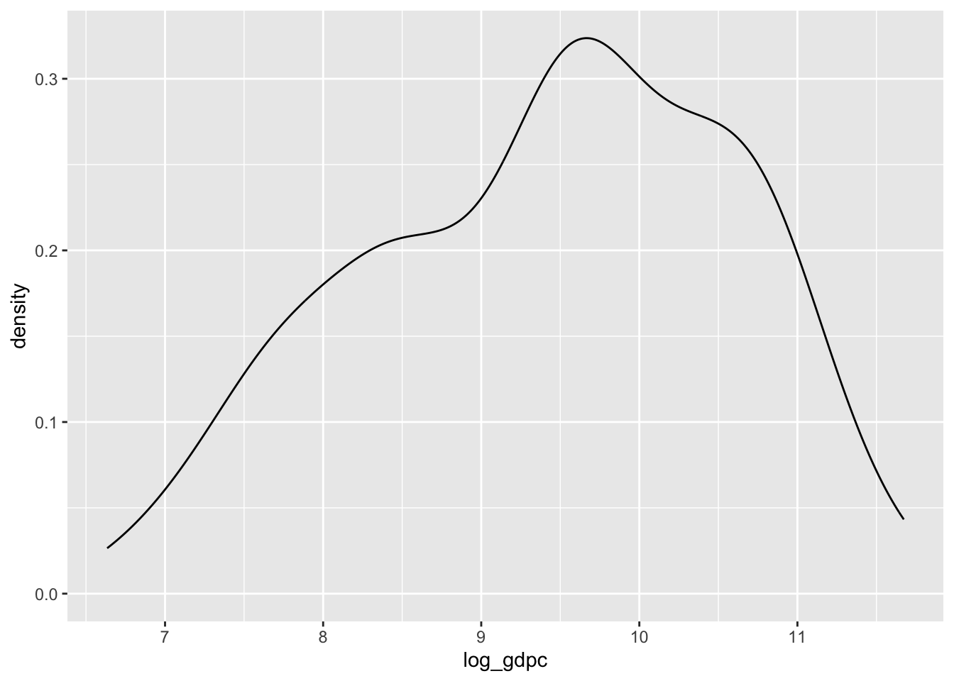
Also showing an over-imposed normal distribution:
fitted_normal <- MASS::fitdistr(na.omit(d$log_gdpc), "normal")$estimate
ggplot(d, aes(x = log_gdpc)) +
  geom_density() +
  stat_function(
    fun = dnorm,
    args = list(mean = fitted_normal[ "mean" ], sd = fitted_normal[ "sd" ]),
    color = "red"
  )
Warning: Removed 11 rows containing non-finite outside the scale range
(`stat_density()`).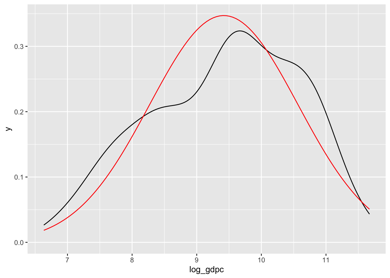
Confidence intervals and standard errors [OPTIONAL]
Why bother with normality? because when a variable is close enough to being normally distributed, the properties of the normal distribution will enable us to compute confidence bounds around its mean (or proportion), through hypothesis tests such as the t-test:
t.test(d$wdi_lifexp)$conf.int[1] 71.23438 73.42240
attr(,"conf.level")
[1] 0.95The result above is not a t-test so to speak: it only shows the ‘95% CI’ (confidence interval) for life expectancy, under the assumption that our data form a random sample of all life expectancy values, and therefore, that its missing values are missing at random
The computation of the interval uses the mean of the variable, its standard deviation, and the sample size, which are used to compute the standard error of the mean (the ‘margin of error’ of average life expectancy):
t.test(d$wdi_lifexp)$stderr[1] 0.5545089There are more formal ways than those above to compute confidence intervals and standard errors in R, which will provide very slightly different results, but ‘hacking’ the t.test function is arguably the quickest way to do so.
Confidence intervals and hypothesis tests are everywhere in statistics; for instance, there are statistical tests for whether a variable is normally distributed with regards to its skewness and kurtosis:
moments::agostino.test(d$log_gdpc) #test of skewness
    D'Agostino skewness test

data:  d$log_gdpc
skew = -0.2992, z = -1.6819, p-value = 0.09258
alternative hypothesis: data have a skewnessmoments::anscombe.test(d$log_gdpc) #test of kurtosis
    Anscombe-Glynn kurtosis test

data:  d$log_gdpc
kurt = 2.2187, z = -3.3743, p-value = 0.00074
alternative hypothesis: kurtosis is not equal to 3
The overall logic of hypothesis testing is not on the menu for today.
Source
Data source
Teorell, Jan, Aksel Sundström, Sören Holmberg, Bo Rothstein, Natalia Alvarado Pachon, Cem Mert Dalli & Yente Meijers. 2023. The Quality of Government Standard Dataset, version Jan23. University of Gothenburg: The Quality of Government Institute, doi:10.18157/qogstdjan23.
Documentation
The codebook of the dataset is available online. Make sure to read it to gain a firm understanding of how the data were assembled and measured.