library(tidyverse) # {dplyr}, {ggplot2}, {readxl}, {stringr}, {tidyr}, etc.Exercise 1: Social democratic capitalism (Kenworthy)
Session 7
This notebook replicates selected figures from Lane Kenworthy’s book, illustrating linear (and nonlinear) correlation while doing so.
Download datasets on your computer
Load data and install useful packages
repository <- "data"library(countrycode)Load the data of the 3 following plots:
# Fig. 2.5: relative poverty and welfare states, 2010-2016
fig25 <- readr::read_tsv(paste0(repository, "/sdc-fig2.5.tsv"))
Rows: 21 Columns: 4
── Column specification ────────────────────────────────────────────────────────
Delimiter: "\t"
chr (2): country, countryabbr_nordic
dbl (2): relativepoverty_2010to2016, publicsocexpends_1980to2015_adj2
ℹ Use `spec()` to retrieve the full column specification for this data.
ℹ Specify the column types or set `show_col_types = FALSE` to quiet this message.head(fig25, 10)# A tibble: 10 × 4
country countryabbr_nordic relativepoverty_2010to2…¹ publicsocexpends_198…²
<chr> <chr> <dbl> <dbl>
1 Australia Asl 21.3 11.3
2 Austria Aus 14.6 20.0
3 Belgium Bel 17.7 17.0
4 Canada Can 20.3 10.4
5 Denmark *Den* 12.5 17.4
6 Finland *Fin* 14.1 17.6
7 France Fr 14.4 17.1
8 Germany Ger 15.7 14.4
9 Ireland Ire 16.5 11.1
10 Italy It 19.4 14.3
# ℹ abbreviated names: ¹relativepoverty_2010to2016,
# ²publicsocexpends_1980to2015_adj2# Fig. 8.11: US Democratic party affiliation advantage by generation, 1972-2016
fig811 <- readr::read_tsv(paste0(repository, "/sdc-fig8.11.tsv"))Rows: 31 Columns: 5
── Column specification ────────────────────────────────────────────────────────
Delimiter: "\t"
dbl (5): year, silent_dem_adv, babyboom_dem_adv, genx_dem_adv, millennial_de...
ℹ Use `spec()` to retrieve the full column specification for this data.
ℹ Specify the column types or set `show_col_types = FALSE` to quiet this message.print(fig811, n = Inf)# A tibble: 31 × 5
year silent_dem_adv babyboom_dem_adv genx_dem_adv millennial_dem_adv
<dbl> <dbl> <dbl> <dbl> <dbl>
1 1972 29.1 35.7 NA NA
2 1973 28.2 23.8 NA NA
3 1974 35.1 32.1 NA NA
4 1975 24 36.7 NA NA
5 1976 33 29.1 NA NA
6 1977 29.9 31.5 NA NA
7 1978 20.5 20.3 NA NA
8 1980 22.6 22.7 NA NA
9 1982 20.5 20.6 NA NA
10 1983 13.6 15.7 NA NA
11 1984 18.3 13.8 NA NA
12 1985 16.6 -0.100 -12.4 NA
13 1986 18 9.5 -9.40 NA
14 1987 18.9 7.70 -9.20 NA
15 1988 11.4 10.9 4.40 NA
16 1989 10.5 2.70 -6 NA
17 1990 13.5 -0.600 -11.6 NA
18 1991 2.90 4.10 -15.3 NA
19 1993 0.800 13.2 -4.30 NA
20 1994 7.20 8.30 1.90 NA
21 1996 4.10 4.80 5.80 NA
22 1998 11 6.5 13.2 NA
23 2000 6.10 10.9 3.70 NA
24 2002 2.10 6.20 7.40 15.6
25 2004 4 3.90 2.30 26.5
26 2006 5.80 8.90 5.80 12.8
27 2008 2.90 9.60 16.3 25.6
28 2010 16.5 10.1 11.3 18.4
29 2012 9.60 14.2 11.6 21.8
30 2014 3.5 11.5 12.7 18.9
31 2016 7.30 10.8 11.3 22.2# Fig. 2.23: public social expenditure in Denmark, 1890-2016
fig223 <- readr::read_tsv(paste0(repository, "/sdc-fig2.23.tsv"))Rows: 127 Columns: 5
── Column specification ────────────────────────────────────────────────────────
Delimiter: "\t"
chr (1): country
dbl (4): year, gdppc, gdppc_log, publicsocexpends
ℹ Use `spec()` to retrieve the full column specification for this data.
ℹ Specify the column types or set `show_col_types = FALSE` to quiet this message.head(fig223, 10)# A tibble: 10 × 5
country year gdppc gdppc_log publicsocexpends
<chr> <dbl> <dbl> <dbl> <dbl>
1 Denmark 1890 4534 8.42 1.11
2 Denmark 1891 4591 8.43 NA
3 Denmark 1892 4668 8.45 NA
4 Denmark 1893 4723 8.46 NA
5 Denmark 1894 4775 8.47 NA
6 Denmark 1895 4978 8.51 NA
7 Denmark 1896 5095 8.54 NA
8 Denmark 1897 5144 8.55 NA
9 Denmark 1898 5156 8.55 NA
10 Denmark 1899 5304 8.58 NA Step 1: understand linear correlation coefficients
Look at the following data preparation:
fig25 <- fig25 %>%
  mutate(
    iso3c = countrycode::countrycode(country, "country.name", "iso3c"),
    region = countrycode::countrycode(country, "country.name", "region"),
    nordic = stringr::str_detect(countryabbr_nordic, "\\*"),
    europe = stringr::str_detect(region, "^Europe"),
    location = case_when(
      nordic ~ "Nordic",
      europe ~ "Europe",
      TRUE ~ "World"
    )
  ) %>%
  dplyr::select(country, iso3c, region, europe, nordic, location,
         poverty = relativepoverty_2010to2016,
         welfare = publicsocexpends_1980to2015_adj2)
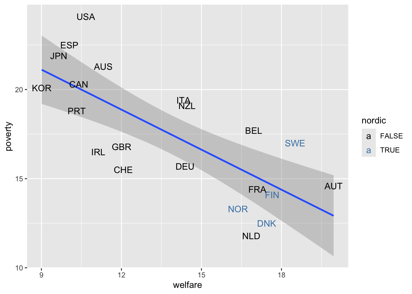
Question 1
Do the following plot which distinguishes Nordic countries.
Clue
See ggplot2::geom_smooth and ggplot2::geom_text and columns poverty and welfare.
The ggplot2::scale_color_manual function helps you to choose the colors you want to use.
Solution
ggplot(fig25, aes(y = poverty, x = welfare)) +
  geom_smooth(method = "lm") +
  geom_text(aes(label = iso3c, colour = nordic)) +
  scale_color_manual(values = c("TRUE" = "steelblue", "FALSE" = "black"))
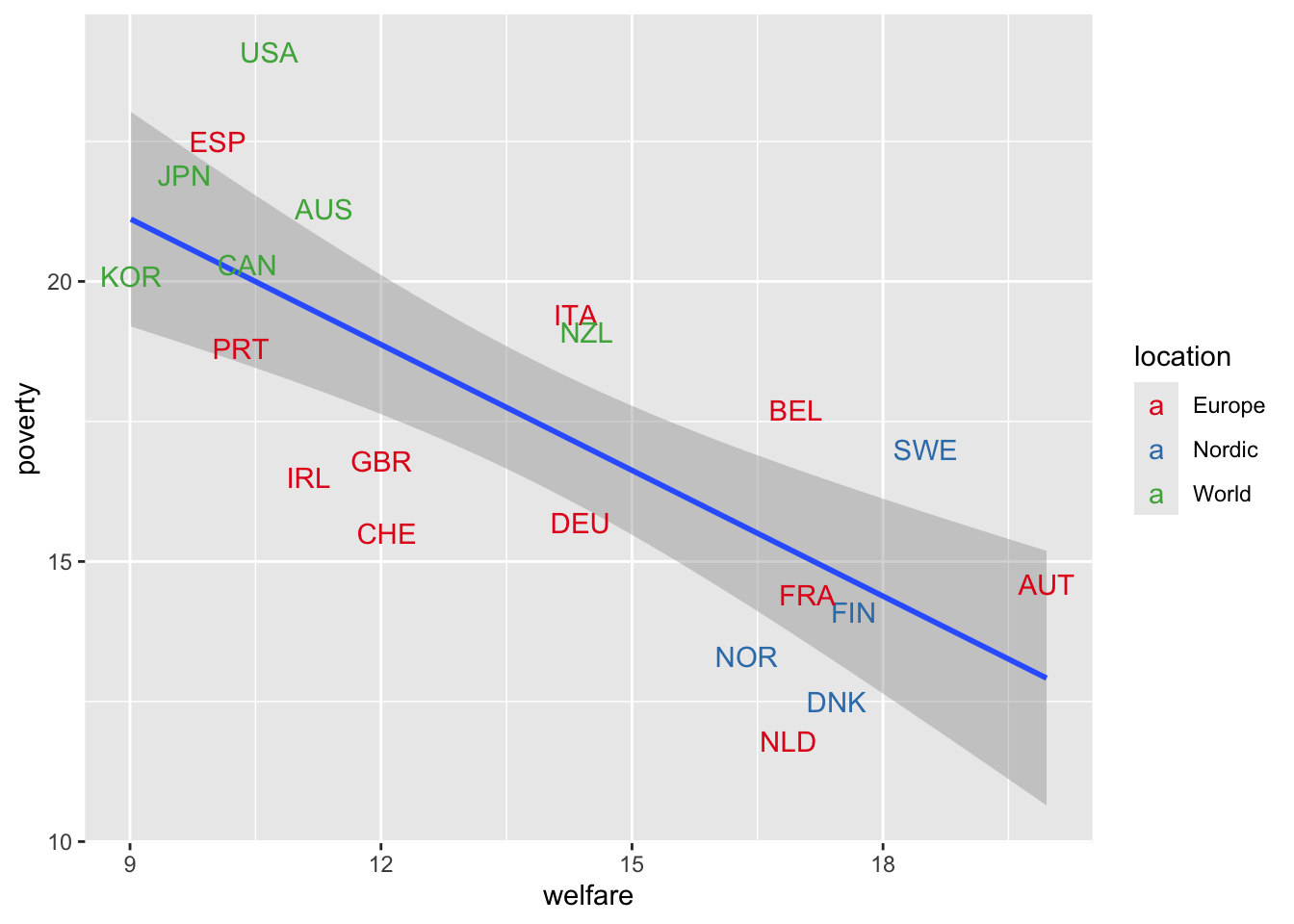
Question 2
Do the following plot which distinguishes Nordic and European countries
Clue
The ggplot2::scale_color_brewer is another way to choose colors, using palettes.
Solution
ggplot(fig25, aes(y = poverty, x = welfare)) +
  geom_smooth(method = "lm") +
  geom_text(aes(label = iso3c, colour = location)) +
  scale_color_brewer(palette = "Set1")
Clue
Simply use the cor function.
Solution
cor(fig25$poverty, fig25$welfare)[1] -0.7402858# equivalent syntax
with(fig25, cor(poverty, welfare)) [1] -0.7402858
Clue
Still use the cor function but think of filtering your dataset before!
Solution
with(fig25 %>% filter(!nordic), cor(poverty, welfare))[1] -0.7050716with(fig25 %>% filter(location == "Europe"), cor(poverty, welfare))[1] -0.6183079with(filter(fig25, location == "World"), cor(poverty, welfare))[1] -0.3856957#Note that in presence of missing data, you will need to use options to select #between pairwise and listwise deletion; what we used above equates to this:
cor(fig25$poverty, fig25$welfare, use = "pairwise.complete.obs")[1] -0.7402858Step 2: Understand pairwise v. listwise case deletion
Look how you remove ‘Democratic advantage’ abbreviation from column names:
fig811 <- fig811 %>% rename_all(~ stringr::str_remove(.x, "_dem_adv"))Write the code to visualize the following time series:
ggplot(pivot_longer(fig811, -year, names_to = "generation") %>%
         mutate(generation = stringr::str_remove(generation, "_dem_adv")),
       aes(year, value, colour = generation)) +
  geom_hline(yintercept = 0, lty = "dashed") +
  geom_point() +
  geom_smooth(method = "loess", se = FALSE)
`geom_smooth()` using formula = 'y ~ x'Warning: Removed 34 rows containing non-finite outside the scale range
(`stat_smooth()`).Warning: Removed 34 rows containing missing values or values outside the scale range
(`geom_point()`).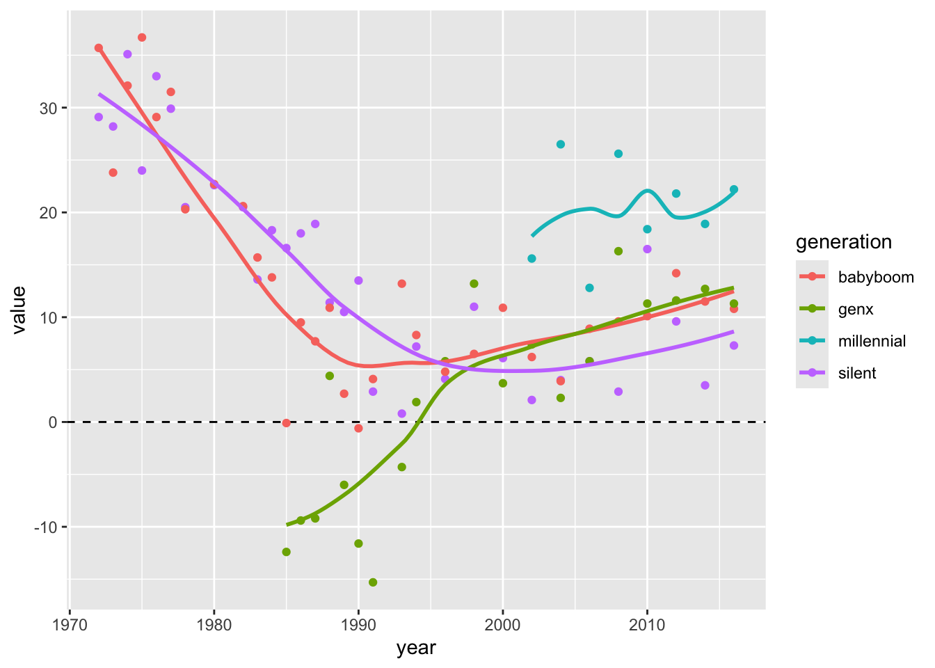
Clue
Still use the cor function.
Solution
use = "everything"(default) includes all variables in the correlation matrix, treating missing values as NA.use = "pairwise"maximizes the use of available data for each pair of variables, making the most of the available information.use = "complete"excludes variables with any missing values from the correlation matrix.
round(cor(fig811), 2) year silent babyboom genx millennial
year 1.00 -0.79 -0.62 NA NA
silent -0.79 1.00 0.77 NA NA
babyboom -0.62 0.77 1.00 NA NA
genx NA NA NA 1 NA
millennial NA NA NA NA 1round(cor(fig811, use = "pairwise"), 2) # pairwise case deletion year silent babyboom genx millennial
year 1.00 -0.79 -0.62 0.82 0.17
silent -0.79 1.00 0.77 -0.35 -0.11
babyboom -0.62 0.77 1.00 0.57 -0.08
genx 0.82 -0.35 0.57 1.00 0.19
millennial 0.17 -0.11 -0.08 0.19 1.00round(cor(fig811, use = "complete"), 2) # listwise case deletion year silent babyboom genx millennial
year 1.00 0.36 0.79 0.61 0.17
silent 0.36 1.00 0.42 0.15 -0.11
babyboom 0.79 0.42 1.00 0.71 -0.08
genx 0.61 0.15 0.71 1.00 0.19
millennial 0.17 -0.11 -0.08 0.19 1.00Step 3: compare linear v. nonlinear trends
Clue
Use dplyr::select and tidyr::drop_na.
Solution
fig223 <- fig223 %>%
  dplyr::select(country, year, socex = publicsocexpends) %>%
  drop_na(socex)
Clue
Still cor!
Solution
cor(fig223$year, fig223$socex)[1] 0.9777574Look at the linear and nonlinear trends:
ggplot(fig223, aes(year, socex)) +
  geom_point() +
  geom_smooth(method = "loess") +
  geom_smooth(method = "lm", se = FALSE, color = "black")
`geom_smooth()` using formula = 'y ~ x'
`geom_smooth()` using formula = 'y ~ x'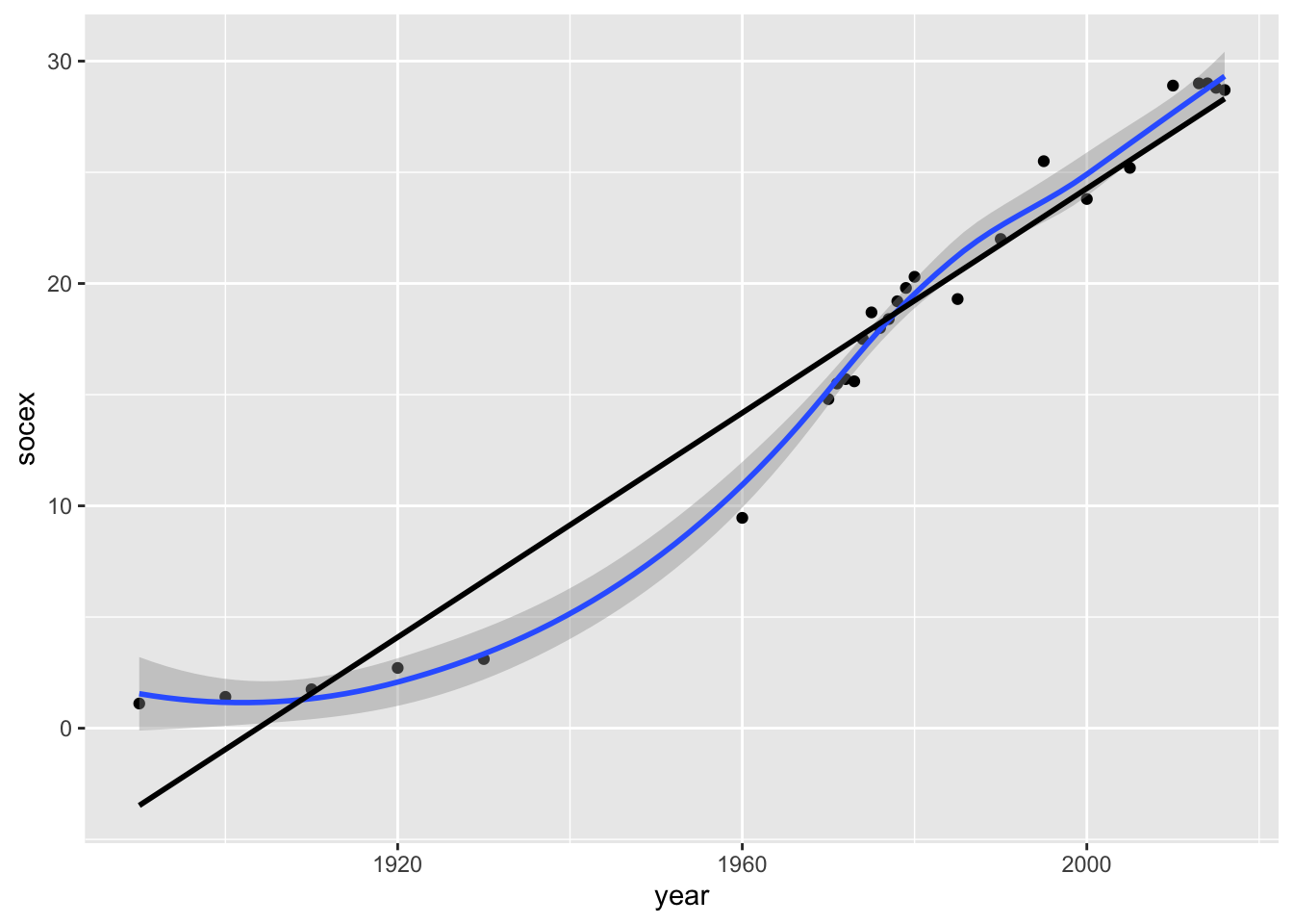
We separate years by historical period:
fig223$period <- cut(fig223$year, c(1889, 1959, 1979, 2016), dig.lab = 4)
table(fig223$period)
(1889,1959] (1959,1979] (1979,2016]
5 11 11 We redraw, showing the periods:
ggplot(fig223, aes(year, socex)) +
geom_smooth(method = "loess", color = "black") +
geom_point(aes(colour = period))`geom_smooth()` using formula = 'y ~ x'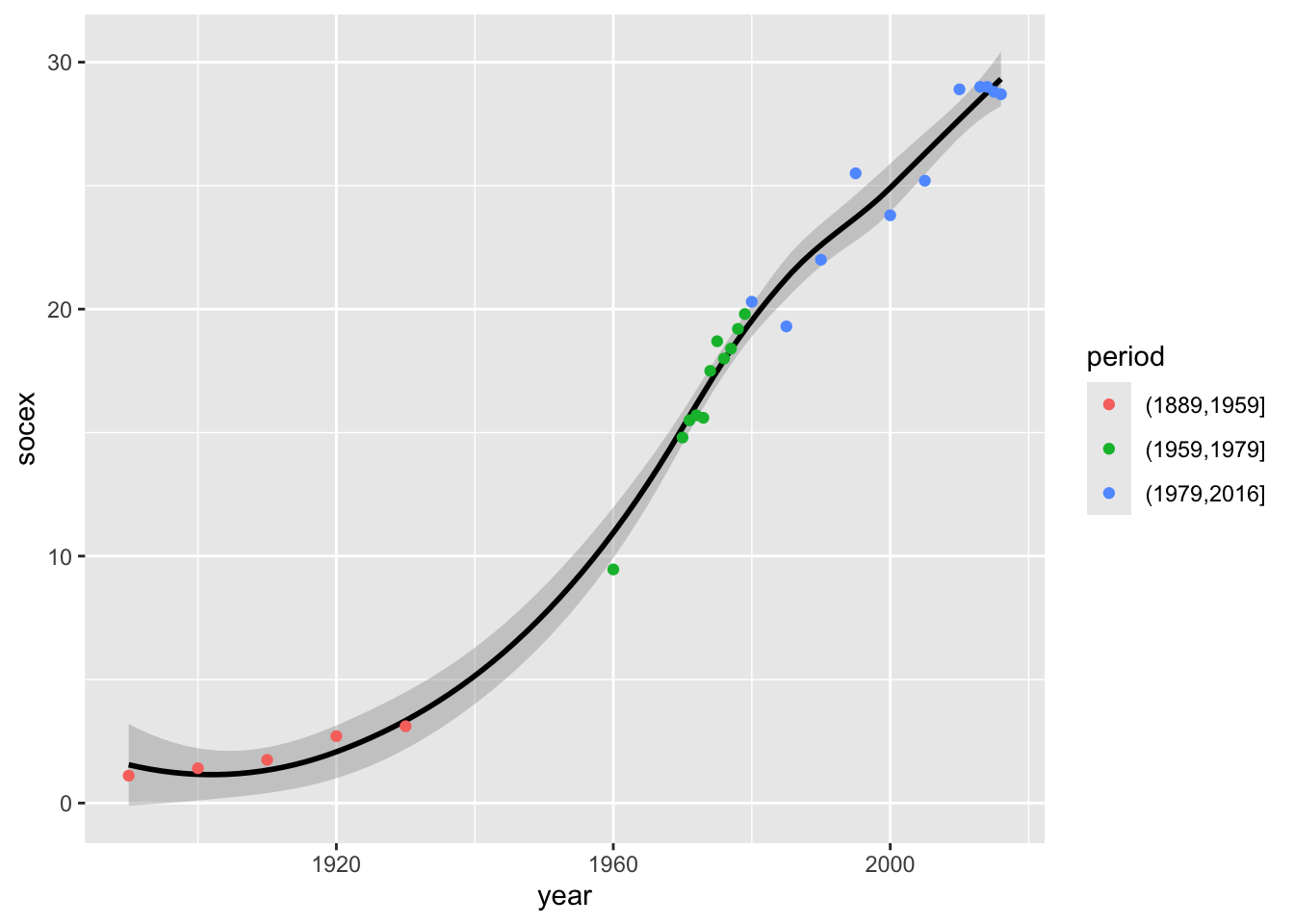
Clue
Still cor!
Solution
corr <- fig223 %>%
group_by(period) %>%
summarise(n = n(),
rho = cor(year, socex)
)
head(corr)
Question 9
Plot the following linear trends for each historical period
`geom_smooth()` using formula = 'y ~ x'
`geom_smooth()` using formula = 'y ~ x'Warning: Removed 48 rows containing missing values or values outside the scale range
(`geom_smooth()`).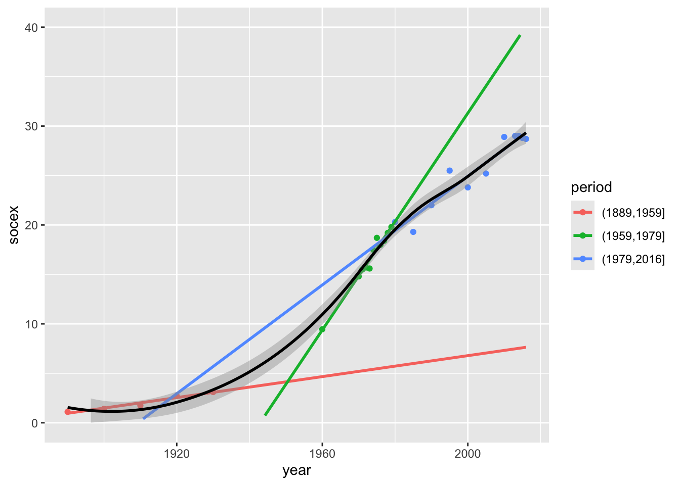
Clue
Use : geom_point, geom_smooth (twice!) and scale_y_continuous.
Solution
ggplot(fig223, aes(year, socex, colour = period)) +
  geom_point() +
  geom_smooth(method = "lm", se = FALSE, fullrange = TRUE) +
  geom_smooth(method = "loess", colour = "black") +
  scale_y_continuous(lim = c(0, 40))
This last graph anticipates on linear regression, since the different slopes here are not correlation coefficients but linear regression coefficients
Step 4: introduction to linear models [OPTIONAL]
No-intercept linear model:
summary(lm(socex ~ year - 1, data = fig223))
Call:
lm(formula = socex ~ year - 1, data = fig223)

Residuals:
    Min      1Q  Median      3Q     Max
-15.819  -2.500   1.010   6.564  10.970

Coefficients:
      Estimate Std. Error t value Pr(>|t|)
year 0.0089569  0.0008542   10.49 7.81e-11 ***
---
Signif. codes:  0 '***' 0.001 '**' 0.01 '*' 0.05 '.' 0.1 ' ' 1

Residual standard error: 8.759 on 26 degrees of freedom
Multiple R-squared:  0.8088,    Adjusted R-squared:  0.8014
F-statistic:   110 on 1 and 26 DF,  p-value: 7.815e-11
Breakdown by historical period:
fig223 %>%
group_by(period) %>%
  # 'restart' year at 0 in each historical period
  mutate(year = year - min(year)) %>%
  # coefficients of no-intercept linear models
  summarise(n = n(), beta = coef(lm(socex ~ year - 1)))
# A tibble: 3 × 3
period n beta
<fct> <int> <dbl>
1 (1889,1959] 5 0.0849
2 (1959,1979] 11 1.17
3 (1979,2016] 11 0.945 Source
Data source
Lane Kenworthy, Social Democratic Capitalism, Oxford University Press, 2020.
R code to generate the sdc-* datasets
The data come directly from Lane Kenworthy’s website, where it is available as an Excel spreadsheet with many tabs.
library(tidyverse)

# Example 1 -- Fig. 2.5
readxl::read_excel("data/sdc-data.xlsx", sheet = "Fig 2.5") %>%
  readr::write_tsv("data/sdc-fig2.5.tsv")

# Example 2 -- Fig. 8.11
readxl::read_excel("data/sdc-data.xlsx", sheet = "Fig 8.11") %>%
  readr::write_tsv("data/sdc-fig8.11.tsv")

# Example 3 -- Fig. 2.23
readxl::read_excel("data/sdc-data.xlsx", sheet = "Fig 2.23") %>%
  readr::write_tsv("data/sdc-fig2.23.tsv")
Unfortunately, the code to replicate either the actual figures of the book, or the data aggregations that underlie many of the plotted series, is not available. The data sources are well detailed in the book, however.