library(tidyverse) # {dplyr}, {ggplot2}, {readxl}, {stringr}, {tidyr}, etc.Exercise 1: Colonialism, democracy, life expectancy and wealth [Part 2]
Session 8
An example inspired by research into the historical legacy of colonialism, using the Quality of Government cross-sectional dataset.
N.B. The course readings can help you if you forgot / don’t know about chi-squared and t tests.
Download datasets on your computer
Step 1: Load data and install useful packages
repository <- "data"# same data as last week, with an additional (geographic) `region` variable
d <- readr::read_tsv(paste0(repository, "/qog2023-extract.tsv"))Rows: 194 Columns: 8
── Column specification ────────────────────────────────────────────────────────
Delimiter: "\t"
chr (3): ccodealp, cname_qog, region
dbl (5): ccode, ht_colonial, br_dem, wdi_lifexp, wdi_gdpcappppcur
ℹ Use `spec()` to retrieve the full column specification for this data.
ℹ Specify the column types or set `show_col_types = FALSE` to quiet this message.Data preparation, replicating the steps we took last week:
d <- d %>%
  mutate(
    former_colony = as.integer(ht_colonial != 0),
    democratic = factor(br_dem, labels = c("Nondemocratic", "Democratic")),
    log_gdpc = log(wdi_gdpcappppcur)
  )
Step 2: cross-tabulation (2 qualitative variables)
Question 1
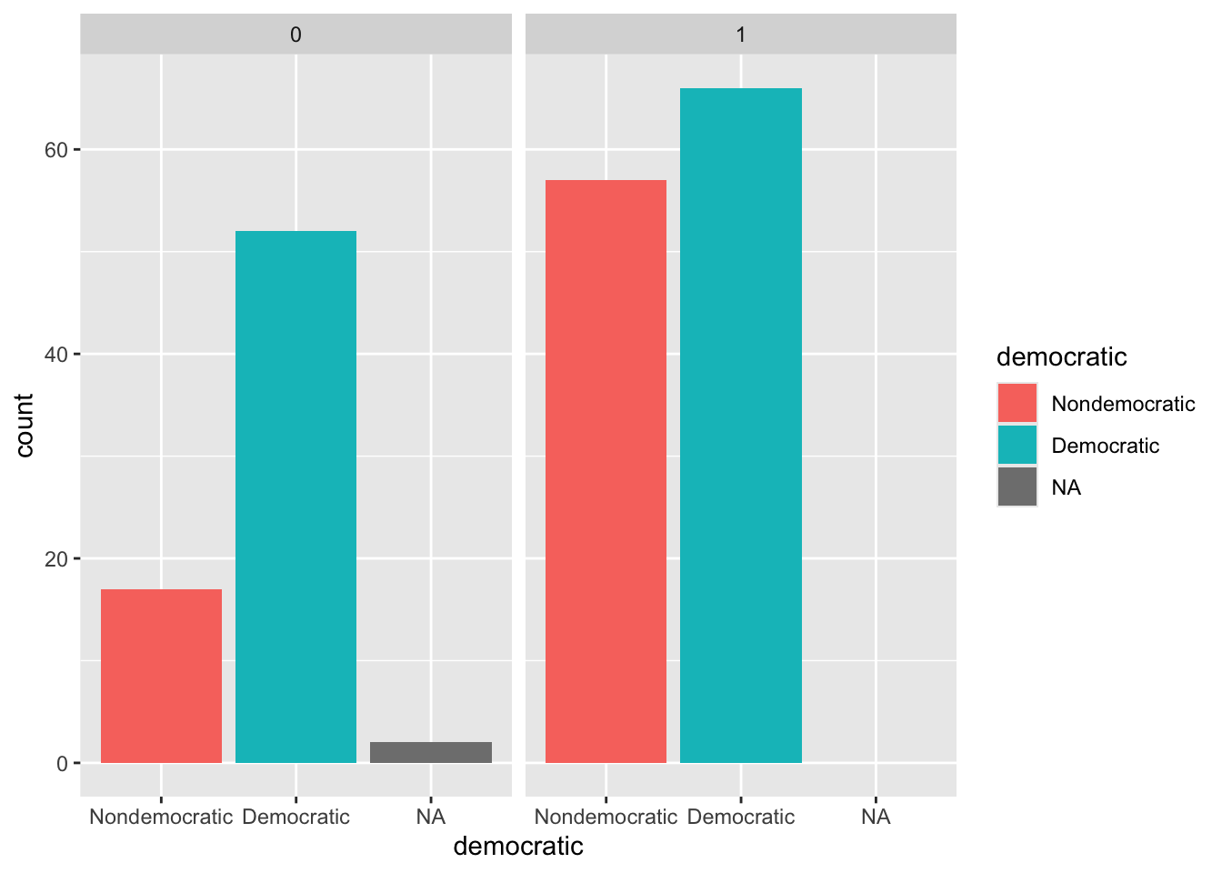
Do the following bar plot of regim (democratic) by (conditional on) colonial origin (former_colony):
Clue
See ggplot2::geom_bar and ggplot2::facet_wrap and columns democratic and former_colony.
Note: The main difference between facet_wrap and facet_grid is that facet_wrap is used for creating a single row or column of subplots whereas facet_grid is used for creating a grid of subplots defined by two categorical variables.
Solution
ggplot(d, aes(x = democratic, fill = democratic)) +
  geom_bar() +
  facet_wrap(~ former_colony)
Clue
See table.
Solution
# Without missing values
t <- table(d$former_colony, d$democratic)
t
    Nondemocratic Democratic
  0            17         52
  1            57         66
# With missing values
t2 <- table(d$former_colony, d$democratic, exclude = NULL)
t2
    Nondemocratic Democratic <NA>
  0            17         52    2
  1            57         66    0
Clue
See prop.table.
Solution
prop.table(t)
    Nondemocratic Democratic
  0    0.08854167 0.27083333
1 0.29687500 0.34375000round(100 * prop.table(t), 1)
    Nondemocratic Democratic
  0           8.9       27.1
1 29.7 34.4prop.table(t, 1) # row percentages
    Nondemocratic Democratic
  0     0.2463768  0.7536232
1 0.4634146 0.5365854prop.table(t, 2) # column percentages
    Nondemocratic Democratic
  0     0.2297297  0.4406780
  1     0.7702703  0.5593220
Clue
See ?chisq.test.
Solution
The purpose of the test is to evaluate how likely the observed frequencies would be assuming the null hypothesis is true.
The null hypothesis is that the two categorical variables are independent.
chisq.test(t)
    Pearson's Chi-squared test with Yates' continuity correction

data:  t
X-squared = 7.8981, df = 1, p-value = 0.004949
p-value < 0.05 so we reject H0. The two variables are dependent
How did we get there?
- Inspect again the relative frequencies of both variables independently
prop.table(table(d$democratic))
Nondemocratic    Democratic
0.3854167 0.6145833 prop.table(table(d$former_colony))
        0         1
0.3659794 0.6340206 - Compare observed versus expected values in the cross tabulation
chisq.test(t)$observed # this is what you observe in your data
    Nondemocratic Democratic
  0            17         52
1 57 66chisq.test(t)$expected # this is what it would look like at random
    Nondemocratic Democratic
  0      26.59375   42.40625
1 47.40625 75.59375- There are less Non-democratic Non-former colony than expected
- There are less Democratic Former colony than expected
- There are more Non-democratic Former colony than expected
- There are more Democratic Non-former colony than expected
=> It seems that there is a link between:
- On the one hand, non-democratic countries and former colonies
- On the other hand, democratic countries and non-former colonies
- Equivalent approach, the Pearson’s residuals:
# Pearson's residuals
chisq.test(t)$residuals
    Nondemocratic Democratic
  0     -1.860367   1.473240
  1      1.393383  -1.103432
When it is negative, the link is positive between the two variables and vice-versa
Step 3: comparison of means (1 quantitative variable + 1 qualitative variable)
Clue
Remember dplyr::group_by and dplyr::summarise.
Solution
d %>%
  group_by(democratic) %>%
  summarise(
    n = n(),
    mean_le = mean(wdi_lifexp, na.rm = TRUE),
    sd_le   =   sd(wdi_lifexp, na.rm = TRUE)
  )
# A tibble: 3 × 4
democratic n mean_le sd_le
<fct> <int> <dbl> <dbl>
1 Nondemocratic 74 69.2 7.11
2 Democratic 118 74.4 7.12
3 <NA> 2 NaN NA The mean of life expectancy seems higher in democratic countries.
You can see visually the following distribution:
ggplot(d %>% drop_na(democratic), aes(x = wdi_lifexp)) +
  geom_density(aes(fill = democratic), alpha = 0.5) +
  geom_rug() +
  scale_fill_brewer("Regime", palette = "Set1") +
  facet_wrap(~ democratic, ncol = 1)
Warning: Removed 7 rows containing non-finite outside the scale range
(`stat_density()`).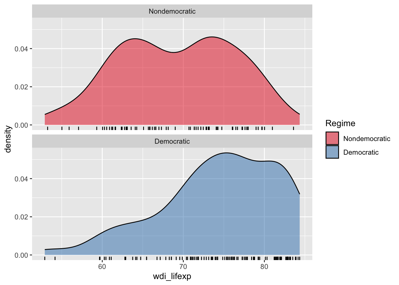
Clue 1
Use the t.test function.
Clue 2
Remember that (H0) No difference in means between group 1 and group 2
Solution
t.test(wdi_lifexp ~ democratic, data = d)
    Welch Two Sample t-test

data:  wdi_lifexp by democratic
t = -4.8891, df = 156.77, p-value = 2.486e-06
alternative hypothesis: true difference in means between group Nondemocratic and group Democratic is not equal to 0
95 percent confidence interval:
 -7.324743 -3.109321
sample estimates:
mean in group Nondemocratic    mean in group Democratic
                   69.19817                    74.41520
“The alternative hypothesis is that the true difference in means between group Nondemocratic and group Democratic is not equal to 0.”
p < 0.05 so the null hypothesis of the equality of mean of life expectancy between the two groups is rejected.
The mean of life expectency is different in democratic versus non-democratic countries.
Going further
Note : The result is “mathematically” complex, breaking it down might help those who want to understand a bit more the mathematical theory (not compulsory)
- Inspect what is in the
t.testobject. A list of different elements
result <- t.test(wdi_lifexp ~ democratic, data = d)
str(result)
List of 10
$ statistic : Named num -4.89
..- attr(*, "names")= chr "t"
$ parameter : Named num 157
..- attr(*, "names")= chr "df"
$ p.value : num 2.49e-06
$ conf.int : num [1:2] -7.32 -3.11
..- attr(*, "conf.level")= num 0.95
$ estimate : Named num [1:2] 69.2 74.4
..- attr(*, "names")= chr [1:2] "mean in group Nondemocratic" "mean in group Democratic"
$ null.value : Named num 0
..- attr(*, "names")= chr "difference in means between group Nondemocratic and group Democratic"
$ stderr : num 1.07
$ alternative: chr "two.sided"
$ method : chr "Welch Two Sample t-test"
$ data.name : chr "wdi_lifexp by democratic"
- attr(*, "class")= chr "htest"- The estimation of the 2 means and their difference.
# difference in means
result$estimate
mean in group Nondemocratic mean in group Democratic
69.19817 74.41520 # not near 0...
result$estimate[1]-result$estimate[2]mean in group Nondemocratic
-5.217032 - You can compute the t statistic.
Once it is determined, you have to read in t-test table the critical value of Student’s t distribution corresponding to the significance level alpha of your choice (0.05). The degrees of freedom used in this test are result$parameter. If the absolute value of the t-test statistics is greater than the critical value, then we reject H0.
# t statistic
t = result$statistic
t
t
-4.889066 # Its formula:
(result$estimate[1]-result$estimate[2]) / result$stderrmean in group Nondemocratic
-4.889066 # Get degrees of freedom
df = result$parameter
df df
156.774 # Get the quantile
quant = qt(0.05, df)
# If abs(t) > q, we reject H0
abs(t)>quant t
TRUE - If the p-value is under
0.05then we reject (H0). It is the case here
# We reject H0
result$p.value
[1] 2.486236e-06- It is confirmed by the fact that
0is not in the confidence interval
result$conf.int[1] -7.324743 -3.109321
attr(,"conf.level")
[1] 0.95Source
Data source
Teorell, Jan, Aksel Sundström, Sören Holmberg, Bo Rothstein, Natalia Alvarado Pachon, Cem Mert Dalli & Yente Meijers. 2023. The Quality of Government Standard Dataset, version Jan23. University of Gothenburg: The Quality of Government Institute, doi:10.18157/qogstdjan23.
Documentation
The codebook of the dataset is available online. Make sure to read it to gain a firm understanding of how the data were assembled and measured.
R code to generate the qog2023-extract dataset
The data are extracted from the cross-sectional QOG Standard dataset, using the R code below:
library(tidyverse)
library(countrycode)

haven::read_dta("qog_std_cs_jan23_stata14.dta") %>%
  mutate(region = countrycode::countrycode(ccodecow, "cown", "region")) %>%
  select(ccode, ccodealp, cname_qog, region,
         ht_colonial, br_dem, wdi_lifexp, wdi_gdpcappppcur) %>%
  readr::write_tsv("qog2023-extract.tsv")
The original dataset appears in the material for the previous session.