Preparation: US Republican vote shares and life expectancy

For Session 8

Authors

Kim Antunez, François Briatte

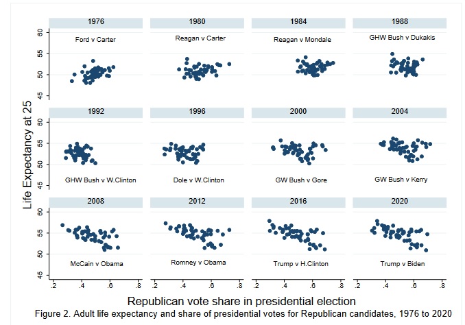
The main goal of this (relatively easy) exercise is to replicate a small part of a recent paper by Anne Case and Angus Deaton. The paper is accessible at the following address:

https://www.nber.org/papers/w29241

The paper was later published in the following journal:

Anne Case and Angus Deaton, “The Great Divide: Education, Despair, and Death,” Annual Review of Economics, vol 14(1), 2022.

Read enough of it to understand the argument behind Figure 2, and to understand the data sources.

Scenario

You are a reviewer for the Annual Review of Economics, and are interested in replicating the authors’ figures in order to check whether they contain any errors.

Instructions

1976-2020-life-expectancy-at-25.csv

This dataset is an extract from the U.S. Mortality Database (HMD). The variables are:

state_po — U.S. state (postal code)
year — year of measurement
lexp25 — life expectancy at 25

As in Case and Deaton’s paper, the 2020 estimate for life expectancy in that dataset is the (most recent) 2018 estimate. Read more on the HMD on its website if needed.

It corresponds to the life expectancy data used by Case and Deaton, with the exacted variables required to replicate Figure 2 of their paper:

repository <- "data"

# life expectancy
le <- readr::read_csv(paste0(repository, "/1976-2020-life-expectancy-at-25.csv"))

Rows: 612 Columns: 3
── Column specification ────────────────────────────────────────────────────────
Delimiter: ","
chr (1): state_po
dbl (2): year, lexp25

ℹ Use `spec()` to retrieve the full column specification for this data.
ℹ Specify the column types or set `show_col_types = FALSE` to quiet this message.

head(le)

# A tibble: 6 × 3
  state_po  year lexp25
  <chr>    <dbl>  <dbl>
1 AK        1976   49.8
2 AK        1980   49.8
3 AK        1984   51.4
4 AK        1988   51.9
5 AK        1992   52.4
6 AK        1996   52.5

If you want, you can find yourself which dataset you need to download from the MIT Election Lab to replicate Figure 2.

Questions

Question 1

What is the mean and standard error of life expectancy of each year of the dataset?

Solution

library(tidyverse) # {dplyr}, {ggplot2}, {readxl}, {stringr}, {tidyr}, etc.

le  %>%
  group_by(year) %>%
  summarise(n = n(),
        mu_lexp = mean(lexp25),
        sd_lexp = sd(lexp25)
  )

# A tibble: 12 × 4
    year     n mu_lexp sd_lexp
   <dbl> <int>   <dbl>   <dbl>
 1  1976    51    50.1    1.19
 2  1980    51    50.8    1.21
 3  1984    51    51.6    1.16
 4  1988    51    51.7    1.44
 5  1992    51    52.5    1.43
 6  1996    51    52.6    1.41
 7  2000    51    53.1    1.39
 8  2004    51    53.8    1.42
 9  2008    51    54.2    1.49
10  2012    51    54.8    1.51
11  2016    51    54.6    1.59
12  2020    51    54.7    1.61

Question 2

Import election data that can be downloaded here:

1976-2020-president.csv

Keep only rows that concern the REPUBLICAN party for which writein == FALSE.

Clue

?dplyr::filter.

Solution

# presidential returns (Republican vote shares)
pr <- readr::read_csv(paste0(repository, "/1976-2020-president.csv"))

Rows: 4287 Columns: 15
── Column specification ────────────────────────────────────────────────────────
Delimiter: ","
chr (6): state, state_po, office, candidate, party_detailed, party_simplified
dbl (7): year, state_fips, state_cen, state_ic, candidatevotes, totalvotes, ...
lgl (2): writein, notes

ℹ Use `spec()` to retrieve the full column specification for this data.
ℹ Specify the column types or set `show_col_types = FALSE` to quiet this message.

head(pr)

# A tibble: 6 × 15
   year state   state_po state_fips state_cen state_ic office       candidate   
  <dbl> <chr>   <chr>         <dbl>     <dbl>    <dbl> <chr>        <chr>       
1  1976 ALABAMA AL                1        63       41 US PRESIDENT "CARTER, JI…
2  1976 ALABAMA AL                1        63       41 US PRESIDENT "FORD, GERA…
3  1976 ALABAMA AL                1        63       41 US PRESIDENT "MADDOX, LE…
4  1976 ALABAMA AL                1        63       41 US PRESIDENT "BUBAR, BEN…
5  1976 ALABAMA AL                1        63       41 US PRESIDENT "HALL, GUS" 
6  1976 ALABAMA AL                1        63       41 US PRESIDENT "MACBRIDE, …
# ℹ 7 more variables: party_detailed <chr>, writein <lgl>,
#   candidatevotes <dbl>, totalvotes <dbl>, version <dbl>, notes <lgl>,
#   party_simplified <chr>

pr <- pr %>%
 filter(party_simplified %in% "REPUBLICAN" & writein==FALSE)
head(pr)

# A tibble: 6 × 15
   year state      state_po state_fips state_cen state_ic office       candidate
  <dbl> <chr>      <chr>         <dbl>     <dbl>    <dbl> <chr>        <chr>    
1  1976 ALABAMA    AL                1        63       41 US PRESIDENT FORD, GE…
2  1976 ALASKA     AK                2        94       81 US PRESIDENT FORD, GE…
3  1976 ARIZONA    AZ                4        86       61 US PRESIDENT FORD, GE…
4  1976 ARKANSAS   AR                5        71       42 US PRESIDENT FORD, GE…
5  1976 CALIFORNIA CA                6        93       71 US PRESIDENT FORD, GE…
6  1976 COLORADO   CO                8        84       62 US PRESIDENT FORD, GE…
# ℹ 7 more variables: party_detailed <chr>, writein <lgl>,
#   candidatevotes <dbl>, totalvotes <dbl>, version <dbl>, notes <lgl>,
#   party_simplified <chr>

Look the problem we have in the dataset for the candidate Mitt Romney.

pr %>% 
  filter(stringr::str_detect(candidate, "ROMNEY")) %>% 
  pull(candidate) %>% table()

.
MITT, ROMNEY ROMNEY, MITT 
           1           50

Let’s correct it!

pr <- pr %>% 
  mutate(candidate = ifelse(stringr::str_detect(candidate, "ROMNEY"),"ROMNEY, MITT",candidate))

Question 3

Compute the vote shares of each candidate.

By year?

By state?

Graphical approaches?

Solution

# compute vote share
pr <- pr %>% mutate(vote_share = candidatevotes / totalvotes)
# or
# pr$vote_share <- pr$candidatevotes / pr$totalvotes

summary(pr$vote_share)

   Min. 1st Qu.  Median    Mean 3rd Qu.    Max. 
 0.0407  0.4203  0.4945  0.4898  0.5693  0.7450

# quick inspection of vote shares by year (candidates shown for reference)
pr %>% group_by(year, candidate) %>%
  summarise(
    n = n(),
    min_vs = min(vote_share),
    mean_vs = mean(vote_share),
    max_vs = max(vote_share)
  ) %>%
  arrange(-mean_vs)

`summarise()` has grouped output by 'year'. You can override using the
`.groups` argument.

# A tibble: 12 × 6
# Groups:   year [12]
    year candidate             n min_vs mean_vs max_vs
   <dbl> <chr>             <int>  <dbl>   <dbl>  <dbl>
 1  1984 REAGAN, RONALD       51 0.137    0.597  0.745
 2  1988 BUSH, GEORGE H.W.    51 0.143    0.537  0.662
 3  2004 BUSH, GEORGE W.      51 0.0934   0.522  0.715
 4  1980 REAGAN, RONALD       51 0.134    0.513  0.728
 5  2020 TRUMP, DONALD J.     50 0.304    0.500  0.695
 6  2000 BUSH, GEORGE W.      51 0.0895   0.496  0.692
 7  2012 ROMNEY, MITT         51 0.0728   0.489  0.728
 8  1976 FORD, GERALD         51 0.165    0.483  0.624
 9  2016 TRUMP, DONALD J.     51 0.0407   0.482  0.686
10  2008 MCCAIN, JOHN         51 0.0653   0.469  0.656
11  1996 DOLE, ROBERT         51 0.0934   0.413  0.544
12  1992 BUSH, GEORGE H.W.    51 0.0910   0.376  0.497

# same thing, graphical approach
ggplot(pr, aes(vote_share, reorder(interaction(year, candidate), vote_share))) +
  geom_boxplot()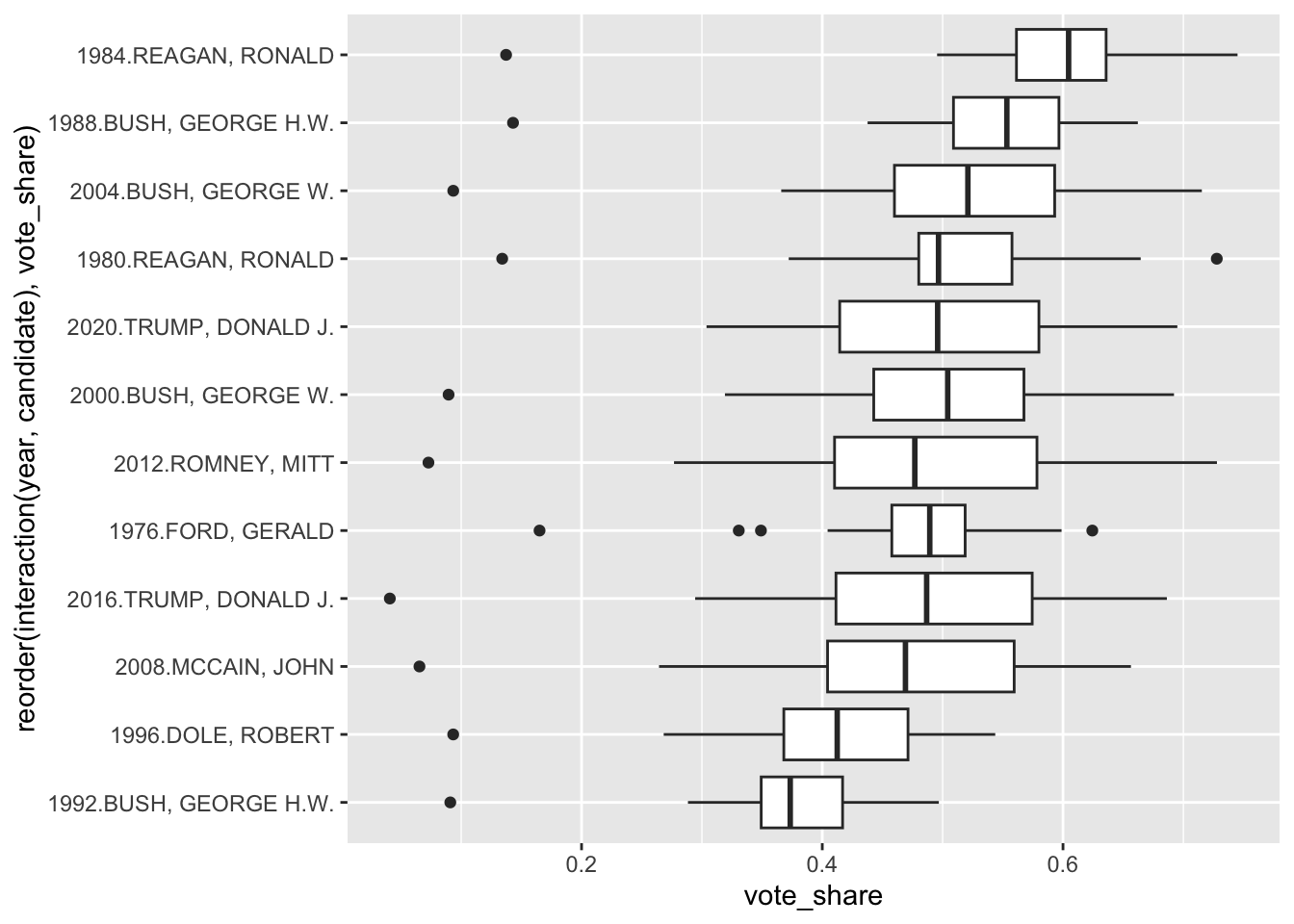

# quick inspection of vote shares by state
pr %>% group_by(state) %>%
  summarise(
    n = n(),
    min_vs = min(vote_share),
    mean_vs = mean(vote_share),
    max_vs = max(vote_share),
    sd_vs = sd(vote_share)
  ) %>%
  arrange(-mean_vs)

# A tibble: 51 × 6
   state            n min_vs mean_vs max_vs  sd_vs
   <chr>        <int>  <dbl>   <dbl>  <dbl>  <dbl>
 1 UTAH            12  0.434   0.626  0.745 0.105 
 2 WYOMING         12  0.397   0.625  0.705 0.0931
 3 IDAHO           12  0.420   0.616  0.724 0.0804
 4 NEBRASKA        12  0.466   0.598  0.706 0.0617
 5 OKLAHOMA        12  0.426   0.597  0.686 0.0844
 6 NORTH DAKOTA    12  0.442   0.576  0.651 0.0719
 7 KANSAS          12  0.389   0.562  0.663 0.0655
 8 ALABAMA         12  0.426   0.561  0.625 0.0688
 9 SOUTH DAKOTA    12  0.407   0.557  0.630 0.0704
10 ALASKA          12  0.395   0.556  0.667 0.0680
# ℹ 41 more rows

# same thing, graphical approach
ggplot(pr, aes(vote_share, reorder(state, vote_share, mean))) +
  geom_boxplot()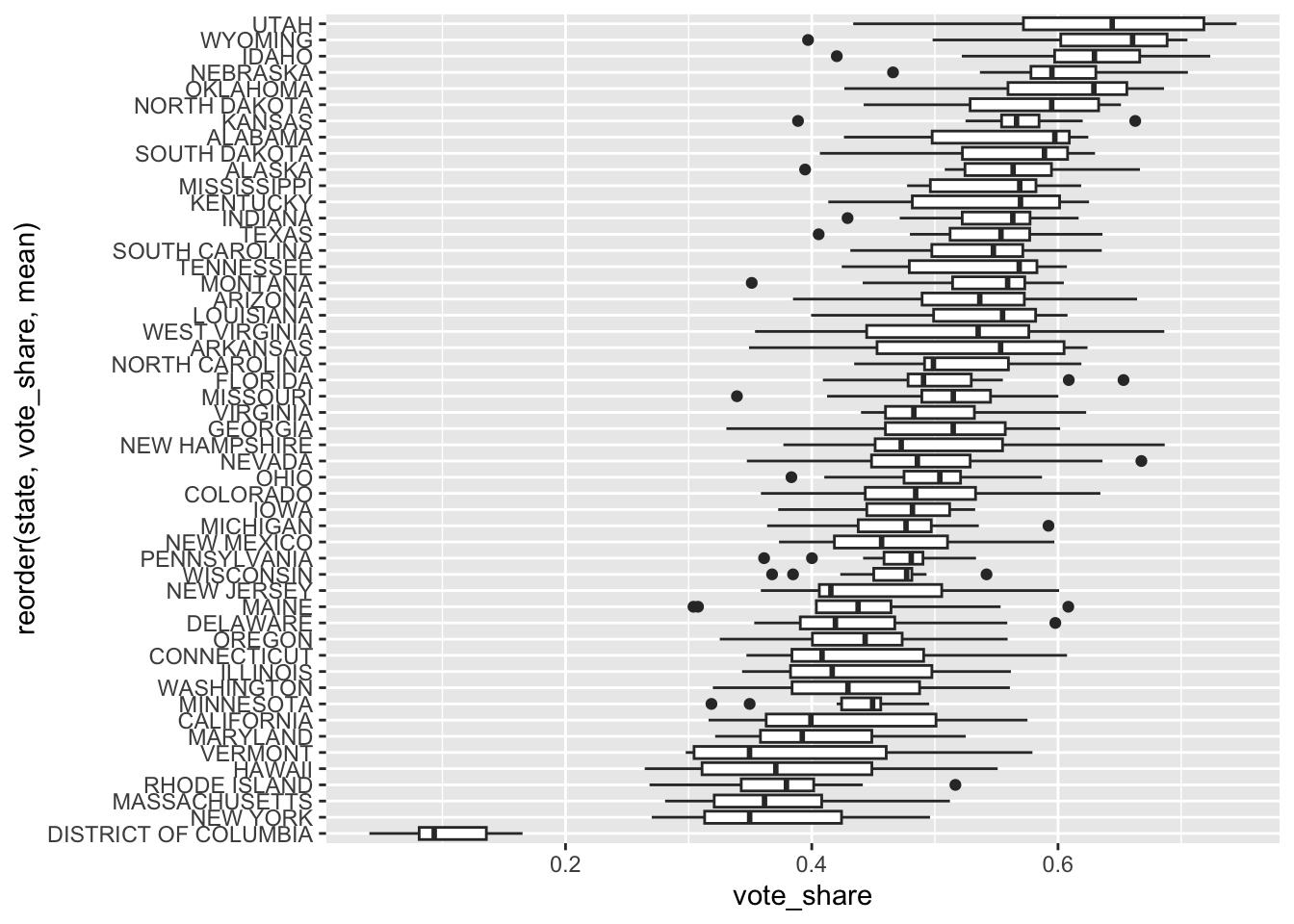

Question 4

Merge the life expectancy and vote shares datasets.

Clue

?dplyr::inner_join (or merge)

Solution

# merge both datasets by year and state
d <- inner_join(le, pr, by = c("year", "state_po"))

Question 5

Replicate Figure 2 to the best of your abilities.

For that, remove the state DC which is an outlier and not in the figures.

`geom_smooth()` using formula = 'y ~ x'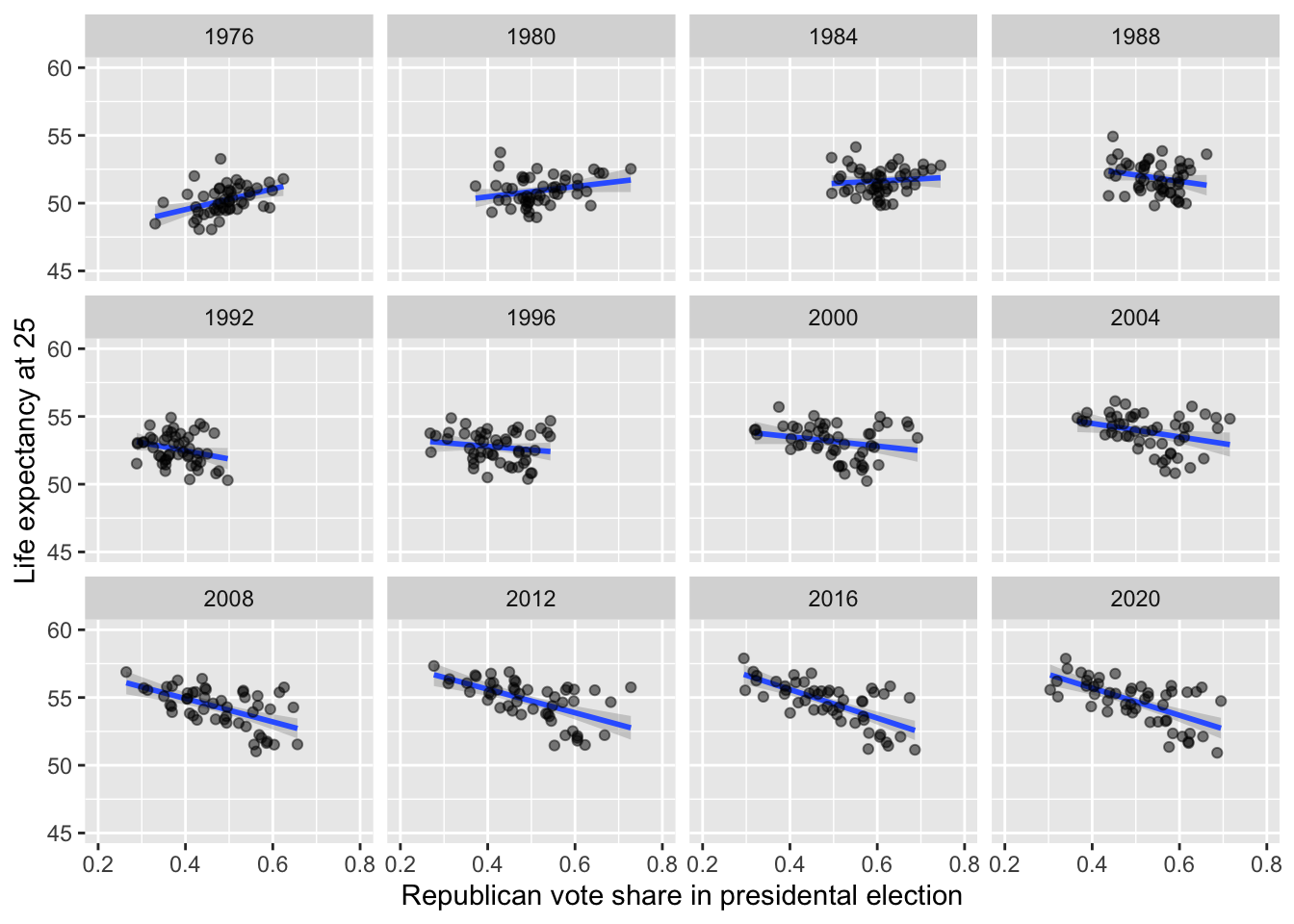

Solution

# something close to Fig. 2
d %>% filter(!state_po %in% "DC") %>%
  ggplot(aes(y = lexp25, x = vote_share)) +
  geom_smooth(method = "lm") +
  geom_point(alpha = 1/2) +
  facet_wrap(~ year) +
  # axis limits used in Fig. 2 (those will exclude DC by design)
  lims(y = c(45, 60), x = c(.2, .8)) +
  # axis titles
  labs(
    y = "Life expectancy at 25",
    x = "Republican vote share in presidental election"
  )

Question 6

How lexp25 and vote_share are correlated to each other?

Assess the following statement, from the authors’ paper:

The interstate correlation goes from +0.42 when Gerald Ford was the Republican candidate—the healthier states voted for Ford and against Carter—to –0.69 in 2016 and –0.64 in 2020 (using 2018 estimates of adult life expectancy). The least healthy states voted for Trump and against Biden.

Solution

# correlation, overall
with(d, cor(lexp25, vote_share))

[1] -0.1031829

# correlation, without DC
with(d %>% filter(!state_po %in% "DC"), cor(lexp25, vote_share))

[1] -0.261351

Negatively correlated, especially without DC.

# correlation, per year (Case and Deaton p. 22)
d %>% filter(!state_po %in% "DC") %>%
  group_by(year) %>%
  summarise(n = n(), rho = round(cor(lexp25, vote_share), 2))

# A tibble: 12 × 3
    year     n   rho
   <dbl> <int> <dbl>
 1  1976    50  0.42
 2  1980    50  0.26
 3  1984    50  0.1 
 4  1988    50 -0.22
 5  1992    50 -0.27
 6  1996    50 -0.16
 7  2000    50 -0.24
 8  2004    50 -0.31
 9  2008    50 -0.57
10  2012    50 -0.59
11  2016    50 -0.69
12  2020    50 -0.64

But the correlation was positive many decades ago!

The numbers in the paper seem correct!

Source

R code to generate the `1976-2020-life-expectancy-at-25` dataset

The code below is provided for reference. You do not need it to complete the exercise.

library(tidyverse)

fs::dir_ls("ushmd-2021-01-07/", glob = "*.csv") %>%
  map_dfr(readr::read_csv, col_types = cols()) %>%
  # get LE for both sexes at 25 for presidential election years + 2018
  filter(Age %in% "25", Year %in% c(seq(1976, 2020, by = 4), 2018)) %>%
  # use 2018 as estimate for LE at 25 in election year 2020
  mutate(year = if_else(Year == 2018, 2020, Year)) %>%
  # keep only useful columns (ex = exact LE at year x = 25)
  select(state_po = PopName, year, lexp25 = ex) %>%
  readr::write_csv("1976-2020-life-expectancy-at-25.csv")

Scenario

Instructions

Questions

Source

R code to generate the 1976-2020-life-expectancy-at-25 dataset

R code to generate the `1976-2020-life-expectancy-at-25` dataset