library(tidyverse) # {dplyr}, {ggplot2}, {readxl}, {stringr}, {tidyr}, etc.Exercise 1: Predicting U.S. presidential election outcomes from income growth
Session 9
An example of how to model electoral performance from just two political fundamentals: economic growth and time in office.
Download datasets on your computer
It is taken from data sent to François Briatte in a personal communication on 30 March 2013. The data is from the 17 presidential elections since the end of World War II and contains the following variables of interest:
incm(dependent variable) : Incumbent (ex-winner) party popular vote margin (%). Example : In 2008, Obama beat McCain by 7.3 percentage points.inc1415(independent variable 1) : Change in real disposable personal income per capita in the second and third quarters of the election year (Q14 and Q15 of the president’s term) : Income Growth, also in percentage points.tenure(independent variable 2) : Years in Office, how long the incumbent (ex-winner) party has held the White House.
Additionnal information based on Wikipedia entries for each presidential election.
Step 1: Load data and install useful packages
library(broom)       # model summaries
library(ggrepel)
library(see) #useful for using performance package
library(patchwork) #useful for using performance package
library(performance) # model performance
library(texreg)      # regression tables
Version: 1.39.3
Date: 2023-11-09
Author: Philip Leifeld (University of Essex)
Consider submitting praise using the praise or praise_interactive functions.
Please cite the JSS article in your publications -- see citation("texreg").repository <- "data"d <- readr::read_csv(paste0(repository,"/bartels4812.csv"))Rows: 17 Columns: 5
── Column specification ────────────────────────────────────────────────────────
Delimiter: ","
dbl (5): year, incm, tenure, inc1415, rdpic
ℹ Use `spec()` to retrieve the full column specification for this data.
ℹ Specify the column types or set `show_col_types = FALSE` to quiet this message.dplyr::glimpse(d)Rows: 17
Columns: 5
$ year <dbl> 1948, 1952, 1956, 1960, 1964, 1968, 1972, 1976, 1980, 1984, 19…
$ incm <dbl> 4.48, -10.85, 15.40, -0.17, 22.58, -0.70, 23.15, -2.06, -9.74,…
$ tenure <dbl> 16, 20, 4, 8, 4, 8, 4, 8, 4, 4, 8, 12, 4, 8, 4, 8, 4
$ inc1415 <dbl> 4.67, 2.42, 0.54, -0.15, 3.35, 1.36, 2.49, 1.26, -0.96, 2.85, …
$ rdpic <dbl> 3.57, 1.49, 3.03, 0.57, 5.74, 3.51, 3.73, 2.98, -0.17, 6.23, 3…p <- readr::read_csv(paste0(repository,"/presidents4820.csv"))Rows: 19 Columns: 6
── Column specification ────────────────────────────────────────────────────────
Delimiter: ","
chr (3): president, party, challenger
dbl (3): year, incumbent, unelected
ℹ Use `spec()` to retrieve the full column specification for this data.
ℹ Specify the column types or set `show_col_types = FALSE` to quiet this message.dplyr::glimpse(p)Rows: 19
Columns: 6
$ year <dbl> 1948, 1952, 1956, 1960, 1964, 1968, 1972, 1976, 1980, 1984,…
$ president <chr> "Truman", "Eisenhower", "Eisenhower", "Kennedy", "Johnson",…
$ party <chr> "Democrat", "Republican", "Republican", "Democrat", "Democr…
$ incumbent <dbl> 1, 0, 1, 0, 1, 0, 1, 0, 1, 1, 0, 1, 1, 0, 1, 0, 1, 0, 0
$ unelected <dbl> 1, 0, 0, 0, 1, 0, 0, 1, 0, 0, 0, 0, 0, 0, 0, 0, 0, 0, 0
$ challenger <chr> "Dewey", "Stevenson", "Stevenson", "Nixon", "Goldwater", "H…We merge the two datasets:
d <- left_join(d, p, by = "year") %>%
  mutate(
    incumbent = as.logical(incumbent),
    incumbent = if_else(incumbent, president, challenger)
  )
head(d)
# A tibble: 6 × 10
year incm tenure inc1415 rdpic president party incumbent unelected
<dbl> <dbl> <dbl> <dbl> <dbl> <chr> <chr> <chr> <dbl>
1 1948 4.48 16 4.67 3.57 Truman Democrat Truman 1
2 1952 -10.8 20 2.42 1.49 Eisenhower Republican Stevenson 0
3 1956 15.4 4 0.54 3.03 Eisenhower Republican Eisenhower 0
4 1960 -0.17 8 -0.15 0.57 Kennedy Democrat Nixon 0
5 1964 22.6 4 3.35 5.74 Johnson Democrat Johnson 1
6 1968 -0.7 8 1.36 3.51 Nixon Republican Humphrey 0
# ℹ 1 more variable: challenger <chr>Step 2: first look at the link between “party vote margin” and “income growth”
# plot
ggplot(d, aes(inc1415, incm)) +
  # horizontal line
  geom_hline(yintercept = 0, lty = "dashed") +
  # data points
  geom_point() +
  # linear correlation with standard error
  geom_smooth(method = "lm") +
  # Label for each point:  incumbent + year
  geom_text(aes(label = stringr::str_c(incumbent, "\n", year))) +
  labs(
    y = "Incumbent party popular vote margin (%)",
    x = "Q14/Q15 growth in real disposable income per capita (%)"
  ) +
  theme_linedraw()
`geom_smooth()` using formula = 'y ~ x'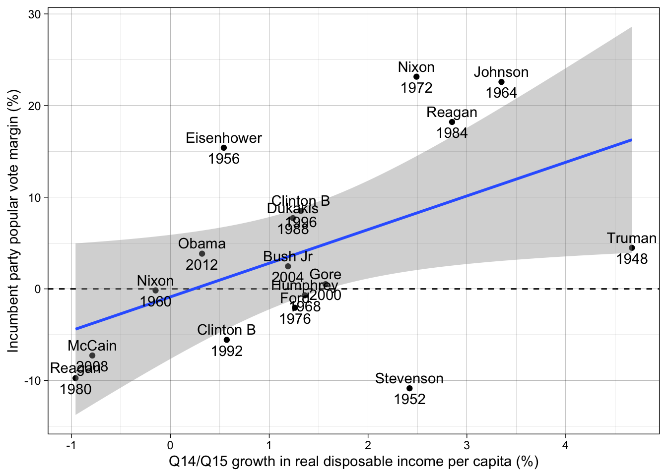
# {ggplot2} global plot theme
theme_set(theme_linedraw())
The same plot observing the “residuals”:
ggplot(broom::augment(lm(incm ~ inc1415, data = d), newdata = d),
       aes(inc1415, incm)) +
  # data points
  geom_point() +
  # linear correlation with standard error
  geom_smooth(method = "lm", fill = "steelblue", alpha = 1/4) +
  # residuals!
  geom_segment(
    aes(y = .fitted, yend = incm, xend = inc1415, color = .resid > 0),
    lty = "dashed"
  ) +
  # fitted values
  geom_point(aes(y = .fitted, x = inc1415), color = "steelblue") +
  ggrepel::geom_text_repel(aes(label = stringr::str_c(incumbent, "\n", year))) +
  scale_color_brewer(palette = "Set1") +
  labs(
    y = "Incumbent party popular vote margin (%)",
    x = "Q14/Q15 growth in real disposable income per capita (%)"
  )
`geom_smooth()` using formula = 'y ~ x'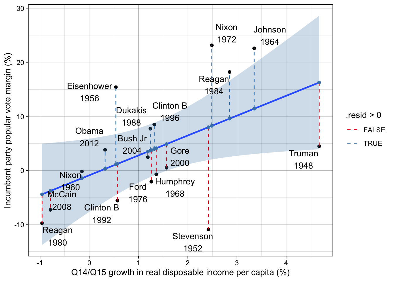
Step 3: simple linear regression
Clue
Use the following syntax:
M1 <- lm(DEPENDANT_VAR ~ INDEPENDANT_VAR, data = DATASET)
summary(M1)
Solution
M1 <- lm(incm ~ inc1415, data = d)
summary(M1)
Call:
lm(formula = incm ~ inc1415, data = d)

Residuals:
    Min      1Q  Median      3Q     Max
-18.860  -5.343  -1.036   4.537  14.883

Coefficients:
            Estimate Std. Error t value Pr(>|t|)
(Intercept)  -0.8726     3.1754  -0.275   0.7872
inc1415       3.6707     1.6104   2.279   0.0377 *
---
Signif. codes:  0 '***' 0.001 '**' 0.01 '*' 0.05 '.' 0.1 ' ' 1

Residual standard error: 9.431 on 15 degrees of freedom
Multiple R-squared:  0.2573,    Adjusted R-squared:  0.2077
F-statistic: 5.196 on 1 and 15 DF,  p-value: 0.0377
Model objects contain many, many results
str(M1)List of 12
$ coefficients : Named num [1:2] -0.873 3.671
..- attr(*, "names")= chr [1:2] "(Intercept)" "inc1415"
$ residuals : Named num [1:17] -11.79 -18.86 14.29 1.25 11.16 ...
..- attr(*, "names")= chr [1:17] "1" "2" "3" "4" ...
$ effects : Named num [1:17] -17.1 -21.5 12.7 -2.16 16.99 ...
..- attr(*, "names")= chr [1:17] "(Intercept)" "inc1415" "" "" ...
$ rank : int 2
$ fitted.values: Named num [1:17] 16.27 8.01 1.11 -1.42 11.42 ...
..- attr(*, "names")= chr [1:17] "1" "2" "3" "4" ...
$ assign : int [1:2] 0 1
$ qr :List of 5
..$ qr : num [1:17, 1:2] -4.123 0.243 0.243 0.243 0.243 ...
.. ..- attr(*, "dimnames")=List of 2
.. .. ..$ : chr [1:17] "1" "2" "3" "4" ...
.. .. ..$ : chr [1:2] "(Intercept)" "inc1415"
.. ..- attr(*, "assign")= int [1:2] 0 1
..$ qraux: num [1:2] 1.24 1.07
..$ pivot: int [1:2] 1 2
..$ tol : num 1e-07
..$ rank : int 2
..- attr(*, "class")= chr "qr"
$ df.residual : int 15
$ xlevels : Named list()
$ call : language lm(formula = incm ~ inc1415, data = d)
$ terms :Classes 'terms', 'formula' language incm ~ inc1415
.. ..- attr(*, "variables")= language list(incm, inc1415)
.. ..- attr(*, "factors")= int [1:2, 1] 0 1
.. .. ..- attr(*, "dimnames")=List of 2
.. .. .. ..$ : chr [1:2] "incm" "inc1415"
.. .. .. ..$ : chr "inc1415"
.. ..- attr(*, "term.labels")= chr "inc1415"
.. ..- attr(*, "order")= int 1
.. ..- attr(*, "intercept")= int 1
.. ..- attr(*, "response")= int 1
.. ..- attr(*, ".Environment")=<environment: R_GlobalEnv>
.. ..- attr(*, "predvars")= language list(incm, inc1415)
.. ..- attr(*, "dataClasses")= Named chr [1:2] "numeric" "numeric"
.. .. ..- attr(*, "names")= chr [1:2] "incm" "inc1415"
$ model :'data.frame': 17 obs. of 2 variables:
..$ incm : num [1:17] 4.48 -10.85 15.4 -0.17 22.58 ...
..$ inc1415: num [1:17] 4.67 2.42 0.54 -0.15 3.35 1.36 2.49 1.26 -0.96 2.85 ...
..- attr(*, "terms")=Classes 'terms', 'formula' language incm ~ inc1415
.. .. ..- attr(*, "variables")= language list(incm, inc1415)
.. .. ..- attr(*, "factors")= int [1:2, 1] 0 1
.. .. .. ..- attr(*, "dimnames")=List of 2
.. .. .. .. ..$ : chr [1:2] "incm" "inc1415"
.. .. .. .. ..$ : chr "inc1415"
.. .. ..- attr(*, "term.labels")= chr "inc1415"
.. .. ..- attr(*, "order")= int 1
.. .. ..- attr(*, "intercept")= int 1
.. .. ..- attr(*, "response")= int 1
.. .. ..- attr(*, ".Environment")=<environment: R_GlobalEnv>
.. .. ..- attr(*, "predvars")= language list(incm, inc1415)
.. .. ..- attr(*, "dataClasses")= Named chr [1:2] "numeric" "numeric"
.. .. .. ..- attr(*, "names")= chr [1:2] "incm" "inc1415"
- attr(*, "class")= chr "lm"Different methods and package exist to extract informations about the regression :
Parameters and uncertainty
- Default extraction methods
# default
coef(M1)
(Intercept) inc1415
-0.8726062 3.6707228 confint(M1) 2.5 % 97.5 %
(Intercept) -7.6407815 5.895569
inc1415 0.2382314 7.103214
Clue
Remember the “margin effect” examples seen in class (Example : effect of surface area on the price of a house).
Solution
In a linear regression, predicting the party vote margin (dependent variable in %) based on the income growth (independent variable in %), a coefficient of 3.67 for income growth means that for each additional percentage of income growth, the party vote margin is expected to increase by 3.67 points of percentages, assuming all other factors in the regression (none here!) remain the same.
- … or, with the {texreg} package
# {texreg}
texreg::screenreg(M1)
====================
             Model 1
--------------------
(Intercept)  -0.87
             (3.18)
inc1415       3.67 *
             (1.61)
--------------------
R^2           0.26
Adj. R^2      0.21
Num. obs.    17
====================
*** p < 0.001; ** p < 0.01; * p < 0.05texreg::screenreg(M1, ci.force = TRUE) # with confidence intervals
==========================
             Model 1
--------------------------
(Intercept)   -0.87
             [-7.10; 5.35]
inc1415        3.67 *
             [ 0.51; 6.83]
--------------------------
R^2            0.26
Adj. R^2       0.21
Num. obs.     17
==========================
* 0 outside the confidence interval.- … or, with the {broom} package
# {broom}
broom::tidy(M1)    # coefficients and standard errors
# A tibble: 2 × 5
term estimate std.error statistic p.value
<chr> <dbl> <dbl> <dbl> <dbl>
1 (Intercept) -0.873 3.18 -0.275 0.787
2 inc1415 3.67 1.61 2.28 0.0377broom::tidy(M1, conf.int = TRUE) # with confidence intervals# A tibble: 2 × 7
term estimate std.error statistic p.value conf.low conf.high
<chr> <dbl> <dbl> <dbl> <dbl> <dbl> <dbl>
1 (Intercept) -0.873 3.18 -0.275 0.787 -7.64 5.90
2 inc1415 3.67 1.61 2.28 0.0377 0.238 7.10Goodness-of-fit
For example, R-squared, RMSE (sigma), BIC
# goodness-of-fit, e.g.
broom::glance(M1)
# A tibble: 1 × 12
r.squared adj.r.squared sigma statistic p.value df logLik AIC BIC
<dbl> <dbl> <dbl> <dbl> <dbl> <dbl> <dbl> <dbl> <dbl>
1 0.257 0.208 9.43 5.20 0.0377 1 -61.2 128. 131.
# ℹ 3 more variables: deviance <dbl>, df.residual <int>, nobs <int>
Clue
You can find explanations of goodness-of-fit coefficients here: ?broom::glance.lm
Solution
This very simple regression model “explains” 26 % of the observed variation in election outcomes.
Predicted values and residuals
# default
fitted(M1)
1 2 3 4 5 6 7
16.2696694 8.0105430 1.1095841 -1.4232146 11.4243152 4.1195768 8.2674936
8 9 10 11 12 13 14
3.7525045 -4.3965001 9.5889538 3.6790901 1.2197058 3.9727479 4.8904286
15 16 17
3.4955539 -3.7724772 0.3020251 residuals(M1) 1 2 3 4 5 6 7
-11.789669 -18.860543 14.290416 1.253215 11.155685 -4.819577 14.882506
8 9 10 11 12 13 14
-5.812505 -5.343500 8.621046 4.040910 -6.779706 4.537252 -4.380429
15 16 17
-1.035554 -3.497523 3.537975 # {broom`}
broom::augment(M1)# A tibble: 17 × 8
incm inc1415 .fitted .resid .hat .sigma .cooksd .std.resid
<dbl> <dbl> <dbl> <dbl> <dbl> <dbl> <dbl> <dbl>
1 4.48 4.67 16.3 -11.8 0.377 8.91 0.758 -1.58
2 -10.8 2.42 8.01 -18.9 0.0911 8.21 0.221 -2.10
3 15.4 0.54 1.11 14.3 0.0788 8.91 0.107 1.58
4 -0.17 -0.15 -1.42 1.25 0.126 9.76 0.00146 0.142
5 22.6 3.35 11.4 11.2 0.173 9.19 0.178 1.30
6 -0.7 1.36 4.12 -4.82 0.0588 9.67 0.00867 -0.527
7 23.2 2.49 8.27 14.9 0.0956 8.82 0.145 1.66
8 -2.06 1.26 3.75 -5.81 0.0592 9.63 0.0127 -0.635
9 -9.74 -0.96 -4.40 -5.34 0.217 9.63 0.0567 -0.640
10 18.2 2.85 9.59 8.62 0.123 9.45 0.0667 0.976
11 7.72 1.24 3.68 4.04 0.0593 9.70 0.00615 0.442
12 -5.56 0.57 1.22 -6.78 0.0774 9.58 0.0235 -0.748
13 8.51 1.32 3.97 4.54 0.0589 9.68 0.00769 0.496
14 0.51 1.57 4.89 -4.38 0.0600 9.69 0.00733 -0.479
15 2.46 1.19 3.50 -1.04 0.0597 9.76 0.000407 -0.113
16 -7.27 -0.79 -3.77 -3.50 0.195 9.71 0.0206 -0.413
17 3.84 0.32 0.302 3.54 0.0908 9.71 0.00773 0.393broom::augment(M1, newdata = d) # original data + fitted values + residuals# A tibble: 17 × 12
year incm tenure inc1415 rdpic president party incumbent unelected
<dbl> <dbl> <dbl> <dbl> <dbl> <chr> <chr> <chr> <dbl>
1 1948 4.48 16 4.67 3.57 Truman Democrat Truman 1
2 1952 -10.8 20 2.42 1.49 Eisenhower Republican Stevenson 0
3 1956 15.4 4 0.54 3.03 Eisenhower Republican Eisenhower 0
4 1960 -0.17 8 -0.15 0.57 Kennedy Democrat Nixon 0
5 1964 22.6 4 3.35 5.74 Johnson Democrat Johnson 1
6 1968 -0.7 8 1.36 3.51 Nixon Republican Humphrey 0
7 1972 23.2 4 2.49 3.73 Nixon Republican Nixon 0
8 1976 -2.06 8 1.26 2.98 Carter Democrat Ford 1
9 1980 -9.74 4 -0.96 -0.17 Reagan Republican Reagan 0
10 1984 18.2 4 2.85 6.23 Reagan Republican Reagan 0
11 1988 7.72 8 1.24 3.37 Bush Sr Republican Dukakis 0
12 1992 -5.56 12 0.57 2.15 Clinton B Democrat Clinton B 0
13 1996 8.51 4 1.32 2.1 Clinton B Democrat Clinton B 0
14 2000 0.51 8 1.57 3.94 Bush Jr Republican Gore 0
15 2004 2.46 4 1.19 2.49 Bush Jr Republican Bush Jr 0
16 2008 -7.27 8 -0.79 1.47 Obama Democrat McCain 0
17 2012 3.84 4 0.32 1.1 Obama Democrat Obama 0
# ℹ 3 more variables: challenger <chr>, .fitted <dbl>, .resid <dbl>
Clue
Work with the residuals of the previous table.
Solution
The best:
broom::augment(M1, newdata = d) %>%
  arrange(abs(.resid)) %>% head(1) %>% select(year, incumbent, .resid)
# A tibble: 1 × 3
year incumbent .resid
<dbl> <chr> <dbl>
1 2004 Bush Jr -1.04The worst:
broom::augment(M1, newdata = d) %>%
  arrange(desc(abs(.resid))) %>% head(1) %>% select(year, incumbent, .resid)
# A tibble: 1 × 3
year incumbent .resid
<dbl> <chr> <dbl>
1 1952 Stevenson -18.9
Clue
summary(model) again.
Solution
summary(M1)
Call:
lm(formula = incm ~ inc1415, data = d)

Residuals:
    Min      1Q  Median      3Q     Max
-18.860  -5.343  -1.036   4.537  14.883

Coefficients:
            Estimate Std. Error t value Pr(>|t|)
(Intercept)  -0.8726     3.1754  -0.275   0.7872
inc1415       3.6707     1.6104   2.279   0.0377 *
---
Signif. codes:  0 '***' 0.001 '**' 0.01 '*' 0.05 '.' 0.1 ' ' 1

Residual standard error: 9.431 on 15 degrees of freedom
Multiple R-squared:  0.2573,    Adjusted R-squared:  0.2077
F-statistic: 5.196 on 1 and 15 DF,  p-value: 0.0377
p-value = 0.04 so yes, the variable is significant at 5 %.
Step 4: regression diagnostics
# distribution of residuals
hist(resid(M1))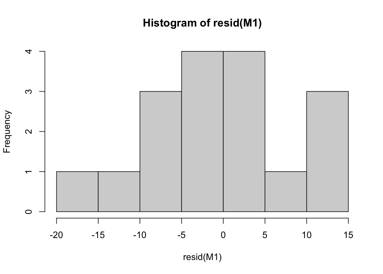
plot(density(residuals(M1)))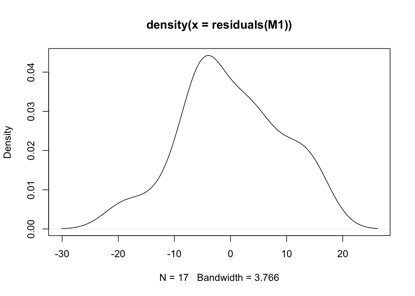
# ... or, with the {ggplot2} package
ggplot(broom::augment(M1), aes(x = .resid)) +
  geom_density(aes(x = .resid))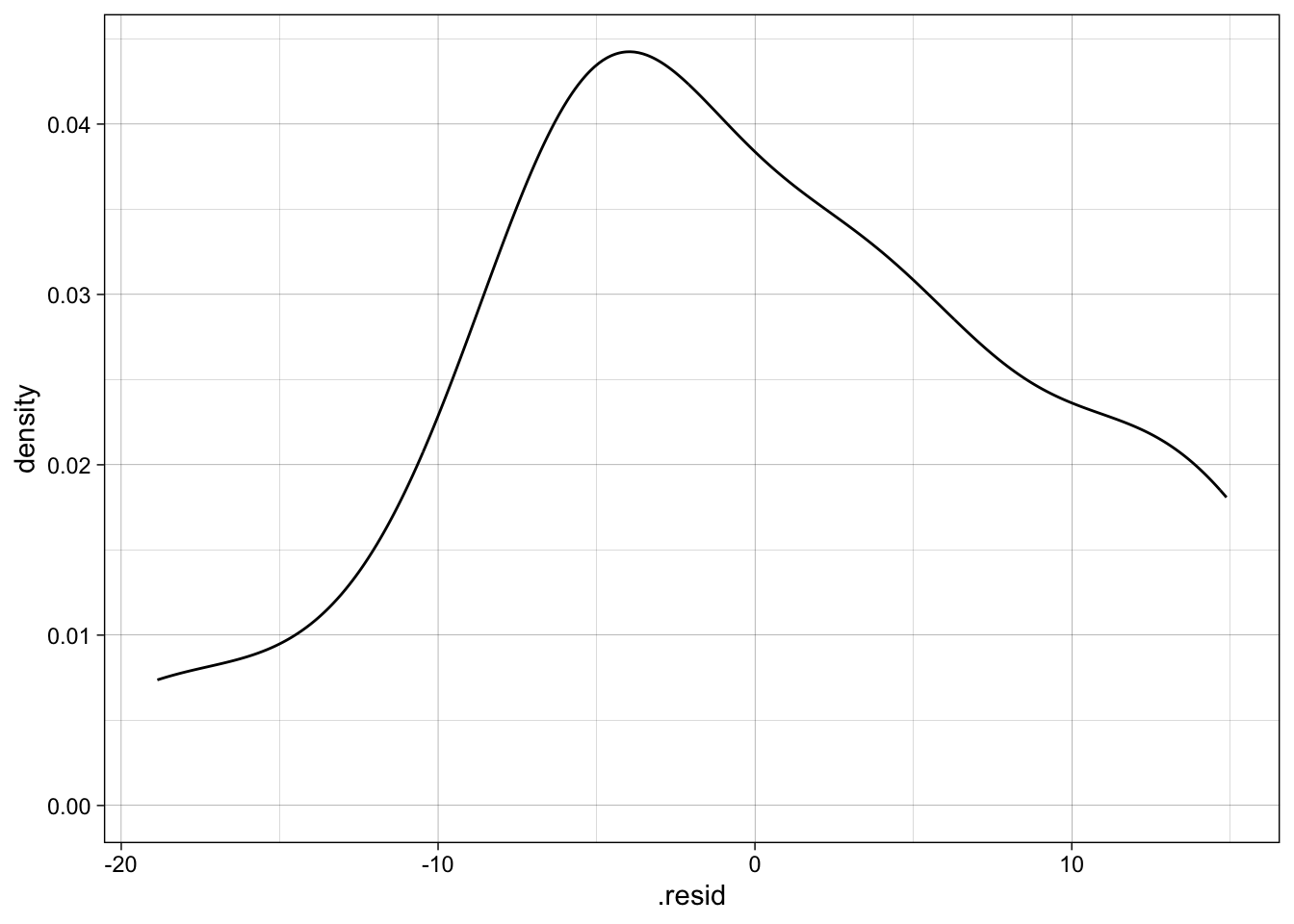
# residuals-versus-fitted values
plot(fitted(M1), residuals(M1))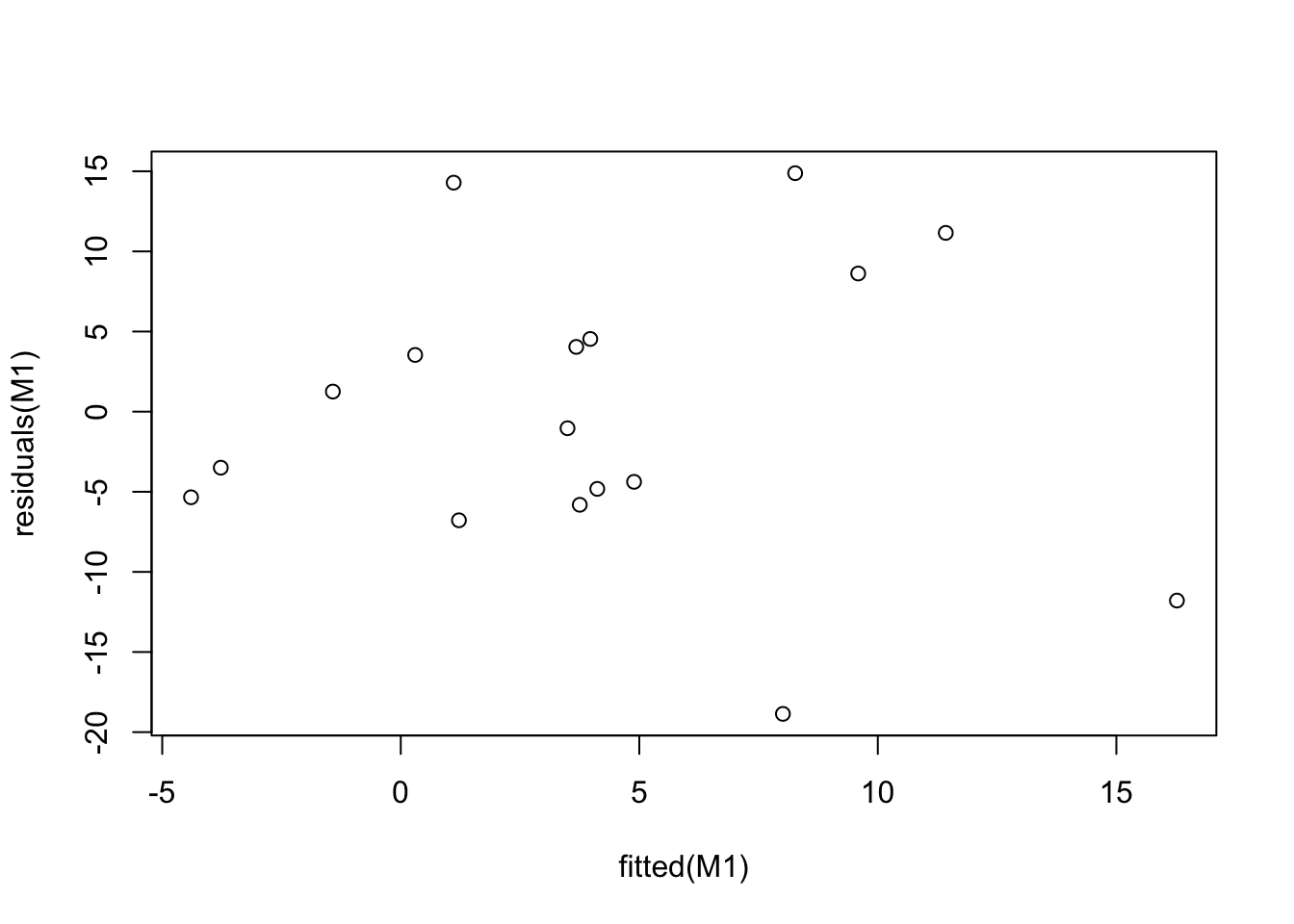
# ... or, with the {ggplot2} package
ggplot(broom::augment(M1, newdata = d)) +
  geom_text(aes(y = .resid, x = .fitted, label = year)) +
  geom_hline(yintercept = 0, lty = "dashed")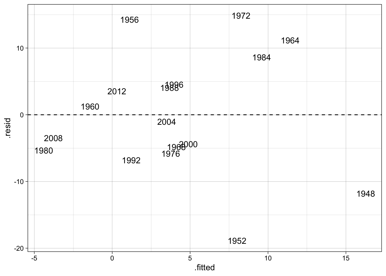
Step 5: multiple linear regression
Clue
Remember the following syntax:
M2 <- lm(DEPENDANT_VAR ~ INDEPENDANT_VAR1 + INDEPENDANT_VAR2, data = DATASET)
summary(M2)
Solution
M2 <- lm(incm ~ inc1415 + tenure, data = d)
summary(M2)
Call:
lm(formula = incm ~ inc1415 + tenure, data = d)

Residuals:
    Min      1Q  Median      3Q     Max
-7.3524 -3.9170 -0.2879  2.5490  9.5650

Coefficients:
            Estimate Std. Error t value Pr(>|t|)
(Intercept)   9.9291     2.4632   4.031  0.00124 **
inc1415       5.4818     0.9193   5.963 3.47e-05 ***
tenure       -1.7636     0.2885  -6.113 2.68e-05 ***
---
Signif. codes:  0 '***' 0.001 '**' 0.01 '*' 0.05 '.' 0.1 ' ' 1

Residual standard error: 5.097 on 14 degrees of freedom
Multiple R-squared:  0.7976,    Adjusted R-squared:  0.7686
F-statistic: 27.58 on 2 and 14 DF,  p-value: 1.393e-05
Notice that now both variables are highly significant (individual p-values very near 0, and the same for the one of the F statistic for the general model).
#The adjusted R-squared statistic is .77
round(summary(M2)$adj.r.squared,2)
[1] 0.77#The standard error of the regression is 5.10
round(summary(M2)$sigma,2)[1] 5.1#The standard errors of the regression parameter estimates are 2.46, 0.92, and 0.29
round(summary(M2)$coefficients[,"Std. Error"], 2)(Intercept) inc1415 tenure
2.46 0.92 0.29 Let’s add a third independent variable and see what happens:
M3 <- lm(incm ~ inc1415 + tenure + unelected, data = d)
summary(M3)
Call:
lm(formula = incm ~ inc1415 + tenure + unelected, data = d)

Residuals:
    Min      1Q  Median      3Q     Max
-7.4906 -2.2260 -0.8544  3.2964  9.3765

Coefficients:
            Estimate Std. Error t value Pr(>|t|)
(Intercept)   9.8107     2.4759   3.962 0.001623 **
inc1415       6.0416     1.0970   5.507 0.000101 ***
tenure       -1.7624     0.2896  -6.085 3.87e-05 ***
unelected    -3.7169     3.9368  -0.944 0.362307
---
Signif. codes:  0 '***' 0.001 '**' 0.01 '*' 0.05 '.' 0.1 ' ' 1

Residual standard error: 5.116 on 13 degrees of freedom
Multiple R-squared:  0.8106,    Adjusted R-squared:  0.7668
F-statistic: 18.54 on 3 and 13 DF,  p-value: 5.591e-05
To compare, the different models:
texreg::screenreg(list(M1, M2, M3))
==========================================
             Model 1  Model 2    Model 3
------------------------------------------
(Intercept)  -0.87     9.93 **    9.81 **
             (3.18)   (2.46)     (2.48)
inc1415       3.67 *   5.48 ***   6.04 ***
             (1.61)   (0.92)     (1.10)
tenure                -1.76 ***  -1.76 ***
                      (0.29)     (0.29)
unelected                        -3.72
                                 (3.94)
------------------------------------------
R^2           0.26     0.80       0.81
Adj. R^2      0.21     0.77       0.77
Num. obs.    17       17         17
==========================================
*** p < 0.001; ** p < 0.01; * p < 0.05
Coefficients plot
# Model 2 only
ggplot(filter(broom::tidy(M2), term != "(Intercept)")) +
  geom_pointrange(
    aes(
      x = term,
      y = estimate,
      ymin = estimate - 1.96 * std.error,
      ymax = estimate + 1.96 * std.error
    )
  ) +
  geom_hline(yintercept = 0, lty = "dashed") +
  coord_flip() # invert y/x axes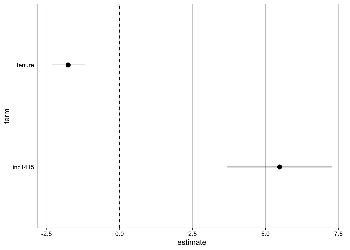
# All models
ggplot(purrr::map_dfr(list(M1, M2, M3), broom::tidy, .id = "model") %>%
         mutate(model = stringr::str_c("M", model)) %>%
         filter(term != "(Intercept)")) +
  geom_pointrange(
    aes(
      x = term,
      y = estimate,
      ymin = estimate - 1.96 * std.error,
      ymax = estimate + 1.96 * std.error,
      color = model
    ),
    position = position_dodge(width = 0.5)
  ) +
  geom_hline(yintercept = 0, lty = "dashed") +
  coord_flip() # invert y/x axes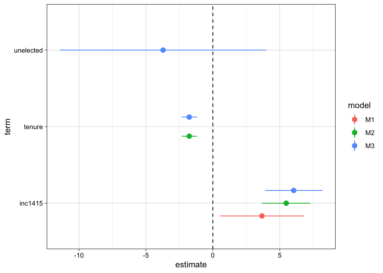
Compare residuals:
ggplot() +
  geom_density(aes(x = resid(M1), fill = "M1", color = "M1"), alpha = 1/3) +
  geom_density(aes(x = resid(M2), fill = "M2", color = "M2"), alpha = 1/3) +
  geom_density(aes(x = resid(M3), fill = "M3", color = "M3"), alpha = 1/3) +
  scale_color_discrete("Model") +
  scale_fill_discrete("Model")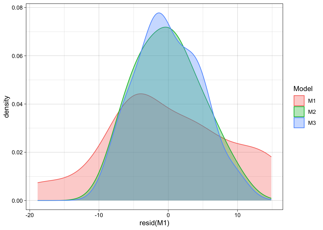
Step 6: Replicate Larry Bartels’ figure [OPTIONAL]
Compute tenure-adjusted effect of real disposable income and replicate Larry Bartels’ Monkey Cage figure (with correct adjustment).
d$inc1415_adjusted <- d$inc1415 + coef(M2)[ "tenure" ] * d$tenure / 4

ggplot(d, aes(inc1415_adjusted, incm)) +
  geom_hline(yintercept = 0, lty = "dashed") +
  geom_smooth(method = "lm") +
  geom_point() +
  geom_text(aes(label = stringr::str_c(incumbent, "\n", year))) +
  labs(y = "Incumbent party popular vote margin (%)",
       x = stringr::str_c("Tenure-adjusted (-1.76 per term) Q14/Q15 growth", "\n",
                 "in real disposable income per capita (%)")) +
  theme_linedraw()
`geom_smooth()` using formula = 'y ~ x'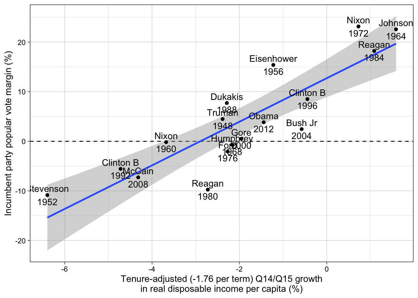
Step 7: further model diagnostics [OPTIONAL]
# model performance, using the `performance` package
performance::model_performance(M2)
# Indices of model performance
AIC | AICc | BIC | R2 | R2 (adj.) | RMSE | Sigma
---------------------------------------------------------------
108.315 | 111.648 | 111.648 | 0.798 | 0.769 | 4.625 | 5.097performance::compare_performance(M1, M2, metrics = "common")# Comparison of Model Performance Indices
Name | Model | AIC (weights) | BIC (weights) | R2 | R2 (adj.) | RMSE
------------------------------------------------------------------------
M1 | lm | 128.4 (<.001) | 130.9 (<.001) | 0.257 | 0.208 | 8.859
M2 | lm | 108.3 (>.999) | 111.6 (>.999) | 0.798 | 0.769 | 4.625# diagnose possible model issues (equivalent to the `car::vif` function)
performance::check_collinearity(M2)# Check for Multicollinearity
Low Correlation
Term VIF VIF 95% CI Increased SE Tolerance Tolerance 95% CI
inc1415 1.12 [1.00, 5.11] 1.06 0.90 [0.20, 1.00]
tenure 1.12 [1.00, 5.11] 1.06 0.90 [0.20, 1.00]performance::check_heteroscedasticity(M2)OK: Error variance appears to be homoscedastic (p = 0.826).performance::check_outliers(M2)OK: No outliers detected.
- Based on the following method and threshold: cook (0.828).
- For variable: (Whole model)# ... or, for even more diagnostics plots (requires installing extra packages)
# install.packages(c("see", "patchwork"))
performance::check_model(M2)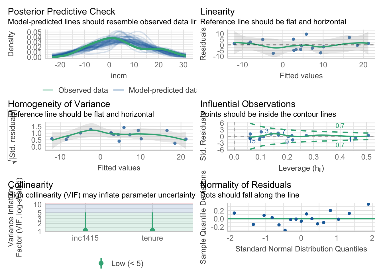
Source
Data source : Larry Bartels, “Obama Toes the Line,” 8 January 2013.
The post contained a figure (not longer available…) and the corresponding equation for it:
Incumbent Party Margin = 9.93 + 5.48 × Income Growth – 1.76 × Years in Office
The demo session for today replicates the model and the figure that comes with it (although the figure in the post uses a different coefficient for Years in office).
See also Christopher Achen and Larry Bartels, Democracy for Realists, Princeton University Press, 2016, ch. 6, or the conference paper cited in the blog post.
The bartels4812 dataset is taken from data sent to François Briatte in a personal communication on 30 March 2013.
The presidents4820 dataset is an addition based on Wikipedia entries for each presidential election.