library(tidyverse) # of simply {dplyr}, {readr}, {ggplot2}.Exam 2: Road traffic accidents in France [dataviz and data analysis]
For Apr. the 30th
In this second exam, you will continue to explore a real-world dataset containing information about road traffic accidents in France in 2022. You’ll perform data visualization and advanced data analysis tasks (distributions, cross-tables, tests, econometrics…) to gain insights from the dataset.
You will be assessed on your ability to manipulate the dataset, apply relevant analysis techniques, and communicate your findings effectively.
This is a graded exercise, to be completed in groups. Make sure to adhere to all ethical and academic integrity standards.
Task 1: Data Preparation
Download datasets
The Etalab database of French road traffic injury accidents for a given year is divided into 4 sections, each represented by a CSV file:
- The CARACTERISTIQUES (CHARACTERISTICS) section that describes the general circumstances of the accident.
- The LIEUX (LOCATIONS) section that describes the main location of the accident, even if it occurred at an intersection.
- The involved VEHICULES (VEHICLES) section.
- The involved USAGERS (USERS) section.
Download the copy of the dataset:
Then, load the required packages and the datasets into R, exactly as you did for exam 1 before.
Solution
repository <- "data"users <- readr::read_delim(paste0(repository, "/usagers-2022.csv"),
show_col_types = FALSE, delim = ";")Warning: One or more parsing issues, call `problems()` on your data frame for details,
e.g.:
dat <- vroom(...)
problems(dat)head(users)# A tibble: 6 × 16
Num_Acc id_usager id_vehicule num_veh place catu grav sexe an_nais trajet
<dbl> <chr> <chr> <chr> <dbl> <dbl> <chr> <chr> <dbl> <chr>
1 2.02e11 1 099 700 813 952 A01 1 1 3 1 2008 5
2 2.02e11 1 099 701 813 953 B01 1 1 1 1 1948 5
3 2.02e11 1 099 698 813 950 B01 1 1 4 1 1988 9
4 2.02e11 1 099 699 813 951 A01 1 1 1 1 1970 4
5 2.02e11 1 099 696 813 948 A01 1 1 1 1 2002 0
6 2.02e11 1 099 697 813 949 B01 1 1 4 2 1987 9
# ℹ 6 more variables: secu1 <chr>, secu2 <chr>, secu3 <chr>, locp <chr>,
# actp <chr>, etatp <chr>Task 2: Age of accidented men versus woman
For this exam, you will focus on the users dataset.
Solution
unique(users$grav)[1] "3" "1" "4" "2" " -1"unique(users$sexe)[1] "1" "2" " -1"users <- users %>%
mutate(grav = ifelse(grav==" -1", NA, grav),
sexe = ifelse(sexe==" -1", NA, sexe))
unique(users$grav)[1] "3" "1" "4" "2" NA unique(users$sexe)[1] "1" "2" NA
Question 2
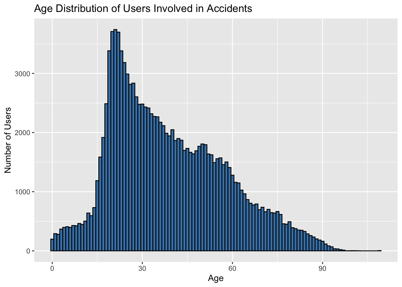
Create a histogram to visualize the age distribution of users involved in accidents.
Solution
# Histogram for age distribution
users <- users %>%
  mutate(age = 2022 - an_nais)

age_distribution_histogram <- users %>%
  filter(!is.na(age)) %>%
  ggplot(aes(x = age)) +
  geom_histogram(binwidth = 1, fill = "steelblue", color = "black") +
  labs(x = "Age", y = "Number of Users", title = "Age Distribution of Users Involved in Accidents")

age_distribution_histogram
Solution
# Average  age of male and female users
average_age_by_gender <- users %>%
  group_by(sexe) %>%
  summarise(average_age = mean(age, na.rm = TRUE)
            )
average_age_by_gender
# A tibble: 3 × 2
sexe average_age
<chr> <dbl>
1 1 38.3
2 2 39.2
3 <NA> 27 38.3 years old for men ; 39.2 for women and 27.0 for missing gender.
# Histogram for age distribution according to gender
age_distribution_histogram_gender <-  users %>%
  filter(!is.na(age)) %>%
  ggplot(aes(x = age, fill=sexe)) +
  geom_histogram(binwidth = 1, color = "black") +
  labs(x = "Age", y = "Number of Users", title = "Age Distribution of Users Involved in Accidents according to gender")

age_distribution_histogram_gender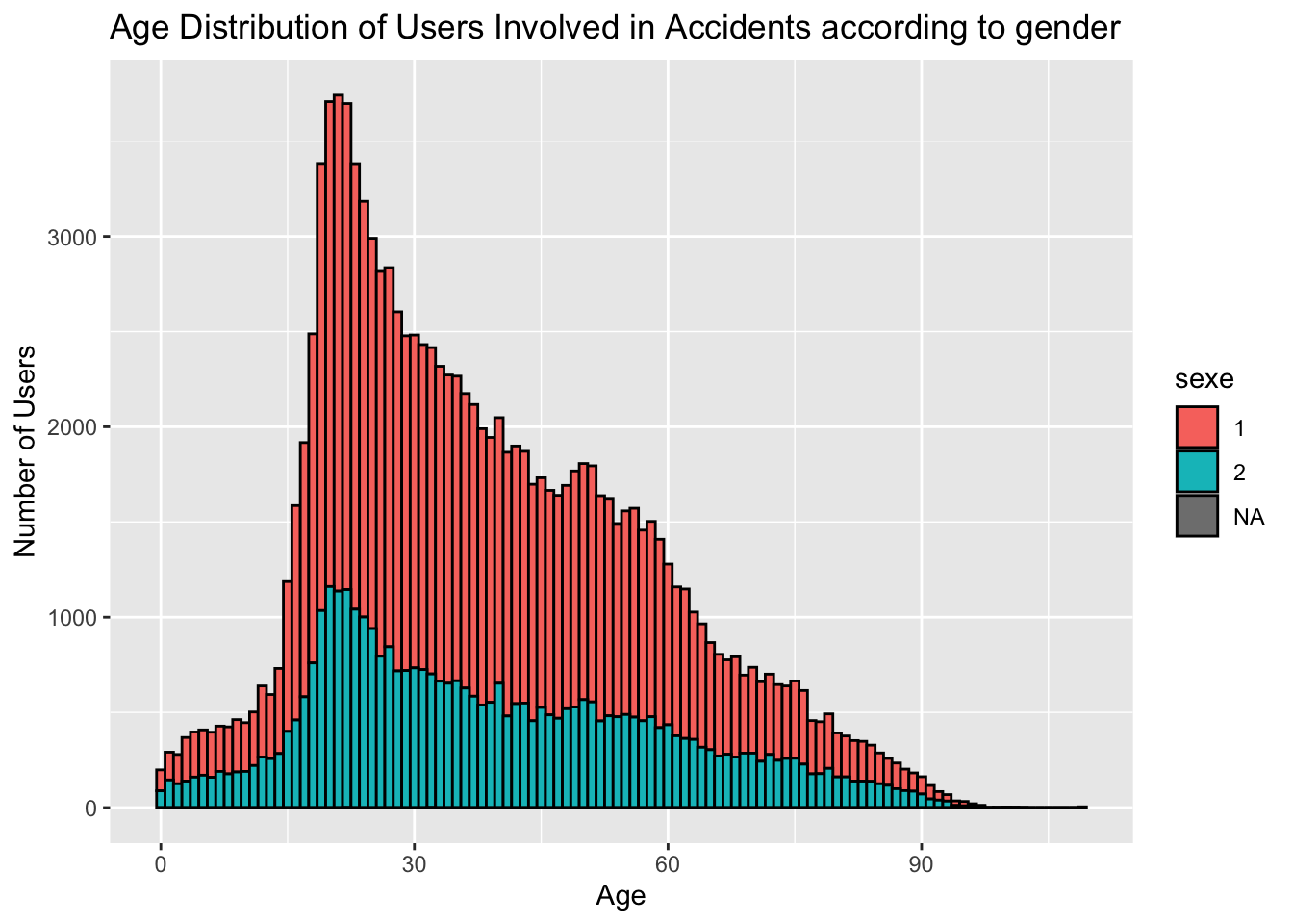
To test if there is (H0) no difference in mean age between accidented male and female, we need to perform a t-test.
t.test(age ~ sexe, data = users)
    Welch Two Sample t-test

data:  age by sexe
t = -7.5517, df = 69530, p-value = 4.348e-14
alternative hypothesis: true difference in means between group 1 and group 2 is not equal to 0
95 percent confidence interval:
 -1.1463502 -0.6739123
sample estimates:
mean in group 1 mean in group 2
       38.27986        39.18999
“The alternative hypothesis is that the true difference in means between groups is not equal to 0.”
p < 0.05 so the null hypothesis of the equality of mean of age between the two groups is rejected.
The mean of age is different for accidented men versus women. More precisely, it is higher for women.
Task 3: Severity, Gender and Age [data analysis]
Solution
# Recoding into factors
users <- users %>%
  mutate(sexe = factor(sexe, levels=c(1,2), labels=c("Male","Female"))) %>%
  mutate(grav = factor(grav, levels=c(1,4,3,2), labels=c("Unhurt","Slight injury","Hospitalized injury","Killed")))

# Cross-tabulation / contingency table between severity and gender
severity_gender_table <- table(users$grav, users$sexe)

# You can see here that men are more accidented than women
colSums(severity_gender_table)
Male Female
84794 39123 You can also calculate proportions of severity versus gender and comment some of them.
100 * prop.table(severity_gender_table)
                            Male     Female
  Unhurt              29.5931954 11.6650661
  Slight injury       25.5945512 14.7397048
  Hospitalized injury 10.9992979  4.5433637
  Killed               2.2410162  0.6238046
29 % of the sample are unhurted men.
100 * prop.table(severity_gender_table, margin = 1)
                          Male   Female
  Unhurt              71.72671 28.27329
  Slight injury       63.45611 36.54389
  Hospitalized injury 70.76843 29.23157
  Killed              78.22535 21.77465
71 % of unhurted people are men.
100 * prop.table(severity_gender_table, margin = 2)
                           Male    Female
  Unhurt              43.247164 36.947576
  Slight injury       37.403590 46.686093
  Hospitalized injury 16.074251 14.390512
  Killed               3.274996  1.975820
Most interesting percentages to interpret the link between the variables. For example : 43 % of accidented men are unhurt versus 37 % of women.
# Chi-squared test for severity and lighting conditions
severity_gender_chisq <- chisq.test(severity_gender_table)
severity_gender_chisq
    Pearson's Chi-squared test

data:  severity_gender_table
X-squared = 1036, df = 3, p-value < 2.2e-16
The purpose of the test is to evaluate how likely the observed frequencies would be assuming the null hypothesis is true. The null hypothesis is that the two categorical variables are independent. p-value < 0.05 so we reject H0. The two variables are dependent
Compare observed versus expected values in the cross tabulation
chisq.test(severity_gender_table)$observed # this is what you observe in your data
                       Male Female
  Unhurt              36671  14455
  Slight injury       31716  18265
  Hospitalized injury 13630   5630
Killed 2777 773chisq.test(severity_gender_table)$expected # this is what it would look like at random
                           Male    Female
  Unhurt              34984.530 16141.470
  Slight injury       34201.029 15779.971
  Hospitalized injury 13179.244  6080.756
Killed 2429.196 1120.804chisq.test(severity_gender_table)$observed - chisq.test(severity_gender_table)$expected
                            Male     Female
  Unhurt               1686.4697 -1686.4697
  Slight injury       -2485.0290  2485.0290
  Hospitalized injury   450.7555  -450.7555
Killed 347.8038 -347.8038- Men are more likely to be Unhurt, Hospitalized or Killed
- Women are more likely to be slightly injured.
Task 4: Severity, Gender and Age [data vizualisation]
Clue
Remember the website The R Graph Gallery – Help and inspiration for R charts
Solution
First a basic grouped box plot:
library(ggplot2)
gg1 <- ggplot(users %>% filter(!is.na(sexe) & !is.na(grav)),
              aes(x = grav, y = age, fill = sexe)) +
  geom_boxplot() +
  labs(title = "Relationship between Age, Gender, and Severity of Accidents",
       x = "Severity",
       y = "Age",
       fill = "Gender") +
  theme_minimal()
gg1
Warning: Removed 132 rows containing non-finite outside the scale range
(`stat_boxplot()`).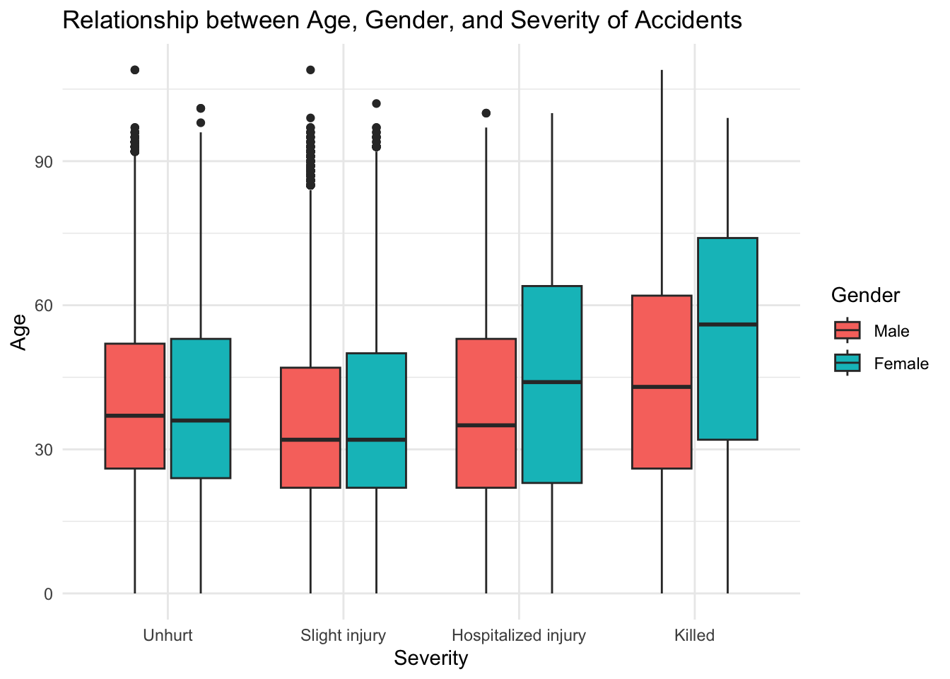
Custom it!
library(ggplot2)
gg2 <- ggplot(users %>% filter(!is.na(sexe) & !is.na(grav)),
              aes(x = grav, y = age, fill = sexe)) +
  geom_boxplot(color = "black", size = 0.7) +
  scale_fill_manual(values = c("#66c2a5", "#fc8d62")) +
  labs(title = "Relationship between Age, Gender, and Severity of Accidents",
       x = "Severity",
       y = "Age",
       fill = "Gender") +
  theme_minimal() +
  theme(text = element_text(size = 12, family = "Arial"),
        plot.title = element_text(face = "bold", hjust = 0.5),
        legend.position = "bottom",
        legend.title = element_text(face = "italic"))
gg2
Warning: Removed 132 rows containing non-finite outside the scale range
(`stat_boxplot()`).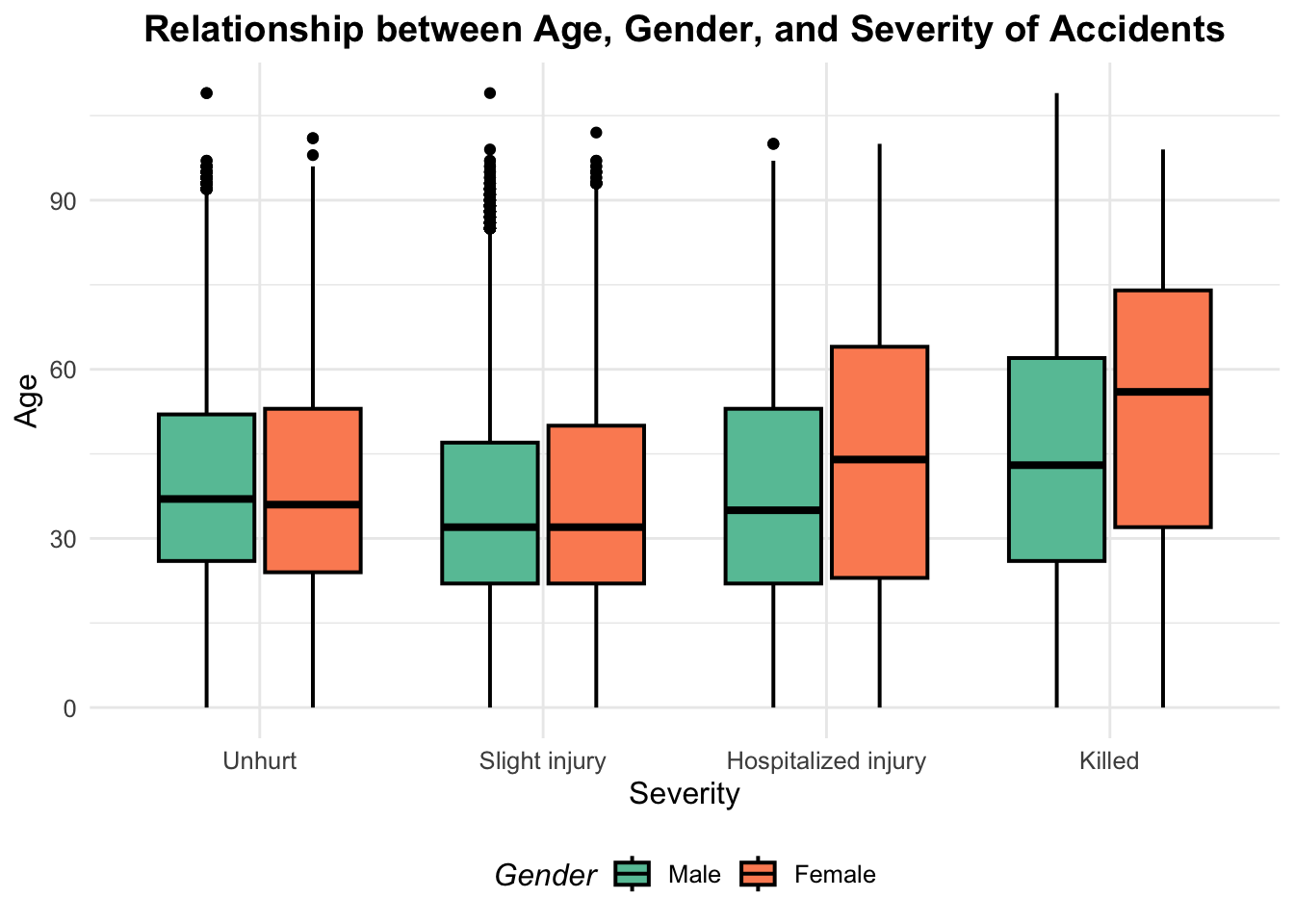
Violin plot. Jitter is not good here because there are two many points!
#https://datavizpyr.com/grouped-violinplot-with-jittered-data-points-in-r/
gg3 <- ggplot(users %>% filter(!is.na(sexe) & !is.na(grav)),
              aes(x = grav, y = age, fill = sexe)) +
  geom_violin(trim = FALSE, color = "black", size = 0.7) +
  geom_point(position = position_jitterdodge(jitter.width = 0.5), size = 0.1, alpha = 0.1, color="lightgrey") +
  scale_fill_manual(values = c("#66c2a5", "#fc8d62")) +
  labs(title = "Relationship between Age, Gender, and Severity of Accidents",
       x = "Severity",
       y = "Age",
       fill = "Gender") +
  theme_minimal() +
  theme(text = element_text(size = 12, family = "Arial"),
        plot.title = element_text(face = "bold", hjust = 0.5),
        legend.position = "bottom",
        legend.title = element_text(face = "italic"))
Warning: Using `size` aesthetic for lines was deprecated in ggplot2 3.4.0.
ℹ Please use `linewidth` instead.gg3Warning: Removed 132 rows containing non-finite outside the scale range
(`stat_ydensity()`).Warning: Removed 132 rows containing missing values or values outside the scale range
(`geom_point()`).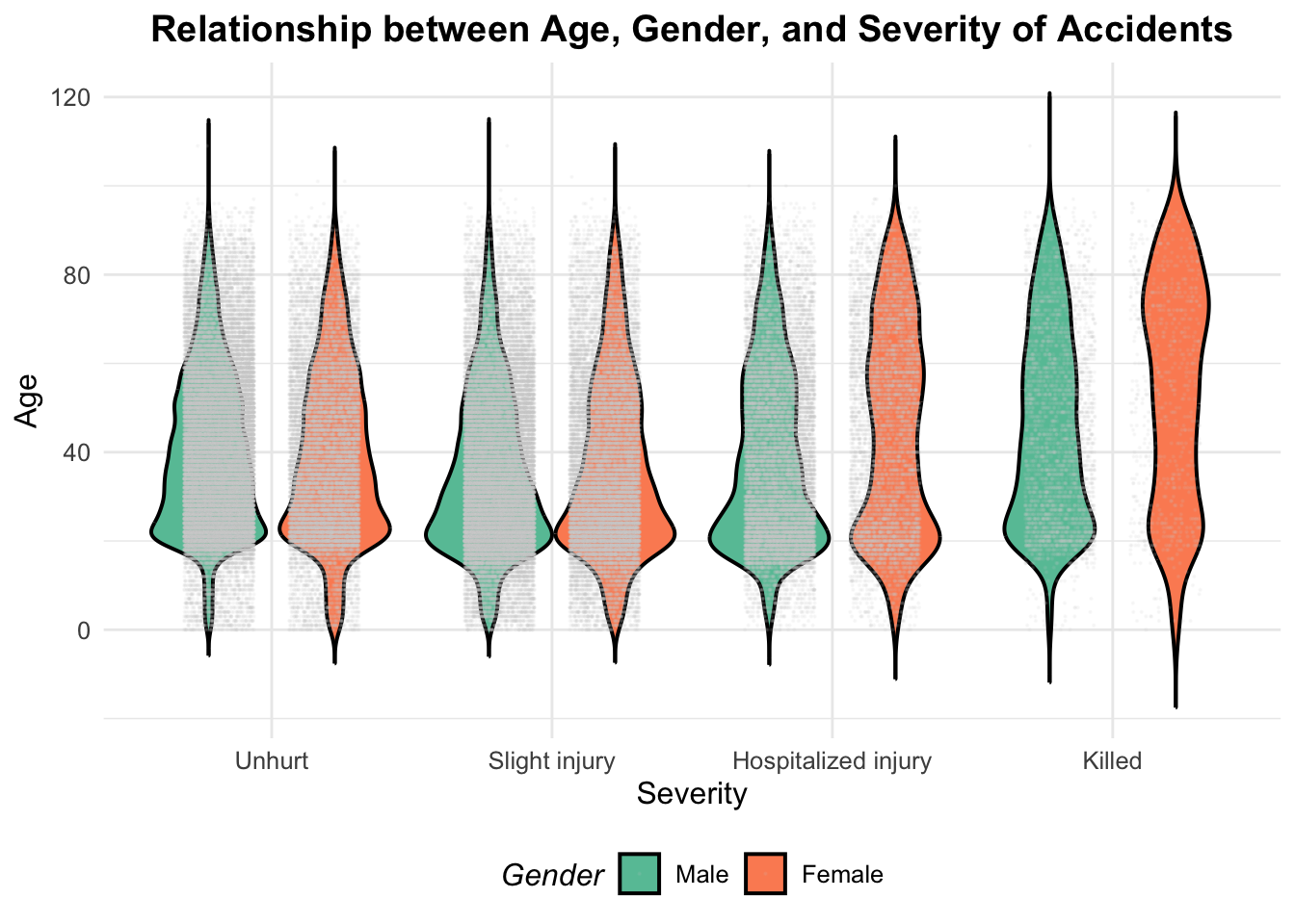
This last plot is very nice because we can see lots of things, such as the fact that among killed woman, the distribution is bimodal: some of them are young (~20 y.o) and others are quite old (~75 y.o).
gg4 <- ggplot(users %>% filter(!is.na(sexe) & !is.na(grav)),
              aes(x = age, y = grav, fill = sexe)) +
  ggridges::geom_density_ridges_gradient(scale = 1, alpha = 0.1) +
  scale_fill_manual(values = c("#66c2a5", "#fc8d62")) +
  facet_wrap("sexe") +
  labs(title = 'Age Distribution by Gender and Severity of Accidents') +
  theme_minimal() +
  theme(
    legend.position = "none",
    panel.spacing = unit(0.1, "lines"),
    strip.text.x = element_text(size = 8)
  ) +
  xlab("Age") +
  ylab("Severity of Accidents")

gg4
Picking joint bandwidth of 2.64Picking joint bandwidth of 3.64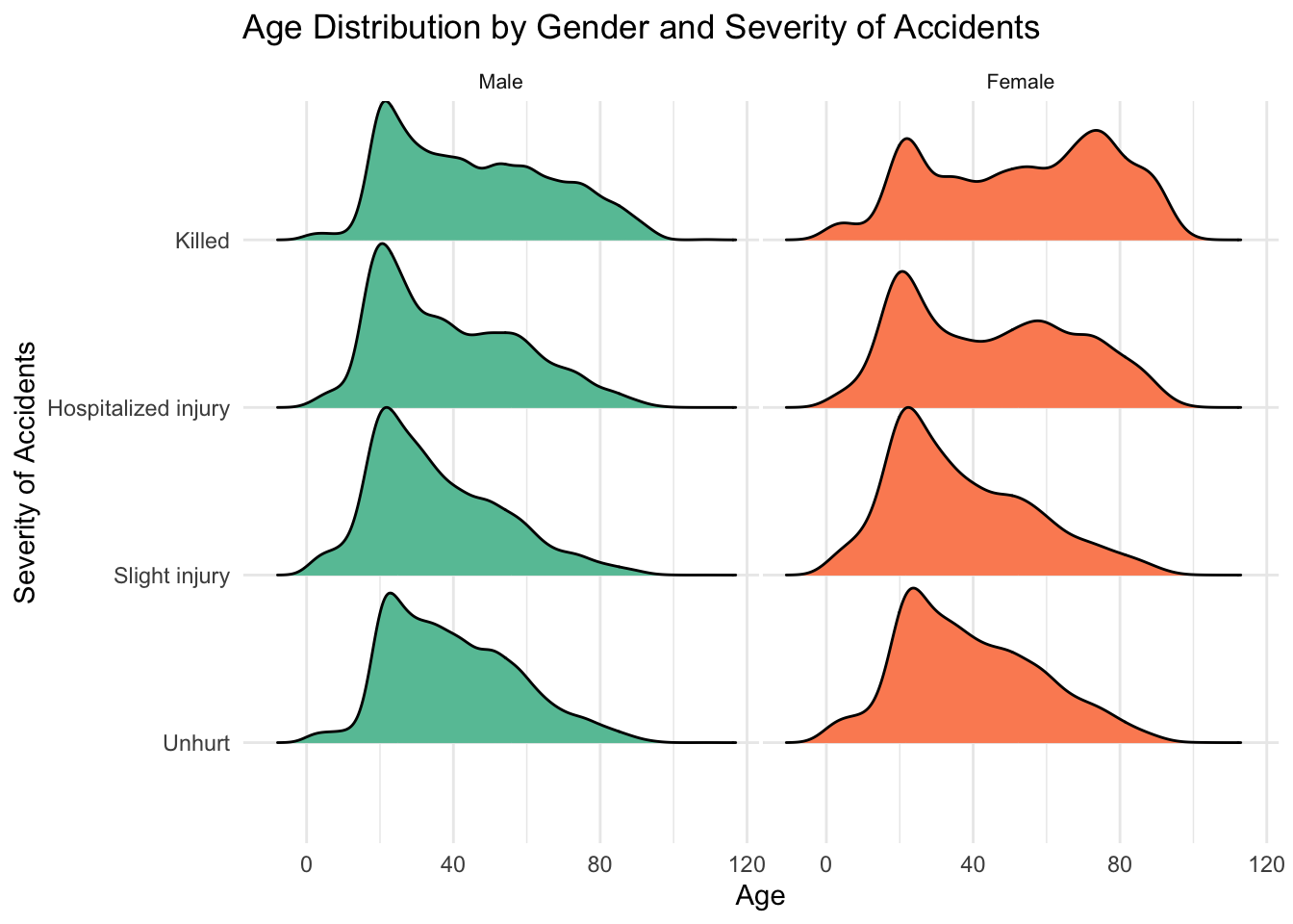
Task 5: Severity, Gender and Age [modeling]
Solution
# Create the killed dummy variable
users <- users %>%
  mutate(killed = ifelse(grav == "Killed",TRUE,FALSE))
M <- glm(killed ~ age + sexe, data = users, family = binomial(link = "logit"))
summary(M)
Call:
glm(formula = killed ~ age + sexe, family = binomial(link = "logit"),
    data = users)

Coefficients:
              Estimate Std. Error z value Pr(>|z|)
(Intercept) -4.3489488  0.0434476 -100.10   <2e-16 ***
age          0.0229222  0.0008443   27.15   <2e-16 ***
sexeFemale  -0.5633427  0.0413179  -13.63   <2e-16 ***
---
Signif. codes:  0 '***' 0.001 '**' 0.01 '*' 0.05 '.' 0.1 ' ' 1

(Dispersion parameter for binomial family taken to be 1)

    Null deviance: 32214  on 123784  degrees of freedom
Residual deviance: 31326  on 123782  degrees of freedom
  (2877 observations deleted due to missingness)
AIC: 31332

Number of Fisher Scoring iterations: 6broom::tidy(M, exponentiate = TRUE)# A tibble: 3 × 5
term estimate std.error statistic p.value
<chr> <dbl> <dbl> <dbl> <dbl>
1 (Intercept) 0.0129 0.0434 -100. 0
2 age 1.02 0.000844 27.2 2.52e-162
3 sexeFemale 0.569 0.0413 -13.6 2.50e- 42All else (i.e gender) being equal, the change in the probability of being killed increases by 2% when the age increases by 1 year.
M_small <- glm(killed ~ age, data = users, family = binomial(link = "logit"))texreg::screenreg(list(M, M_small))
============================================
                Model 1        Model 2
--------------------------------------------
(Intercept)         -4.35 ***      -4.47 ***
                    (0.04)         (0.04)
age                  0.02 ***       0.02 ***
                    (0.00)         (0.00)
sexeFemale          -0.56 ***
                    (0.04)
--------------------------------------------
AIC              31331.57       31533.55
BIC              31360.75       31553.01
Log Likelihood  -15662.79      -15764.78
Deviance         31325.57       31529.55
Num. obs.       123785         123787
============================================
*** p < 0.001; ** p < 0.01; * p < 0.05
AIC is lower in M (Model 1) than M_small (Model 2) : M is a better model. So including the gender in the model seems to improve the quality of the prediction.
In addition, the variable sexe is highly significant.
Submission
Submit your completed exam2_solution.R script via email to kim.antunez@sciencespo.fr by the specified deadline. Use the email subject: “DSR Exam 2 Submission” and detail the names of the students.
Make sure your script is well-organized. It should include clear and concise code, comments explaining your approach, and visualizations (if required).
The answers of the questions must be added in comments using the following syntax:
##############################
## Task 1: Data Preparation ##
##############################

##### Question 1

library(hello)
1+1
# Answer : The average value is 2
Source
The data is obtained on this page.
Variable Dictionary - USAGERS Section
Here is the description of the variables in english. The description in French is in this document
Num_Acc: Accident identifier, identical to the one in the “CARACTERISTIQUES” section, for each user involved in the accident.
id_usager: Unique identifier of the user (including pedestrians attached to vehicles that hit them) - Numeric code.
id_vehicule: Unique identifier of the vehicle for each user occupying it (including pedestrians attached to vehicles that hit them) - Numeric code.
num_Veh: Vehicle identifier for each user occupying it (including pedestrians attached to vehicles that hit them) - Alphanumeric code.
place: Indicates the seat occupied by the user in the vehicle at the time of the accident. Details are given in the document in French.
catu: User category:
- 1 - Driver
- 2 - Passenger
- 3 - Pedestrian
grav: Severity of the user’s injury, classified into three categories of victims plus the unhurt:
- 1 - Unhurt
- 2 - Killed
- 3 - Hospitalized injury
- 4 - Slight injury
sexe: Gender of the user:
- 1 - Male
- 2 - Female
- -1 - Not specified
An_nais: Year of birth of the user.
trajet: Reason for the journey at the time of the accident:
- -1 - Not specified
- 0 - Not specified
- 1 - Home - Work
- 2 - Home - School
- 3 - Errands - Shopping
- 4 - Professional use
- 5 - Leisure - Recreation
- 9 - Other
secu1, secu2, secu3: Safety equipment used by the user until 2018, now indicating usage with up to three possible safety devices for a single user (especially for motorcyclists who are required to wear helmets and gloves).
- -1 - Not specified
- 0 - No equipment
- 1 - Seatbelt
- 2 - Helmet
- 3 - Child device
- 4 - Reflective vest
- 5 - Airbag (2RM/3RM)
- 6 - Gloves (2RM/3RM)
- 7 - Gloves + Airbag (2RM/3RM)
- 8 - Not determinable
- 9 - Other
locp: Pedestrian location:
- -1 - Not specified
- 0 - Not applicable
- On road:
- 1 - A + 50 m from pedestrian crossing
- 2 - A - 50 m from pedestrian crossing
- On pedestrian crossing:
- 3 - No light signal
- 4 - With light signal
- Miscellaneous:
- 5 - On sidewalk
- 6 - On shoulder
- 7 - On refuge or BAU
- 8 - On counter lane
- 9 - Unknown
actp: Pedestrian action:
- -1 - Not specified
- Moving:
- 0 - Not specified or not applicable
- 1 - In the direction of the striking vehicle
- 2 - In the opposite direction of the vehicle
- Miscellaneous:
- 3 - Crossing
- 4 - Masked
- 5 - Playing - Running
- 6 - With animal
- 9 - Other
- A - Getting in/out of vehicle
- B - Unknown
etatp: This variable specifies whether the injured pedestrian was alone or not:
- -1 - Not specified
- 1 - Alone
- 2 - Accompanied
- 3 - In a group