library(tidyverse) # {dplyr}, {ggplot2}, {readxl}, {stringr}, {tidyr}, etc.Exercise 1: Opposition to abortion in Canada, 2021
Session 10
An example of how to model binary responses, a.k.a. probabilities.
Download datasets on your computer
Step 1: Load data and install useful packages
library(broom)       # model summaries
library(texreg)      # regression tables
Version: 1.39.3
Date: 2023-11-09
Author: Philip Leifeld (University of Essex)
Consider submitting praise using the praise or praise_interactive functions.
Please cite the JSS article in your publications -- see citation("texreg").
Attaching package: 'texreg'The following object is masked from 'package:tidyr':
extractlibrary(performance) # model performance
library(effects) #for ggeffects belowLoading required package: carDatalattice theme set by effectsTheme()
See ?effectsTheme for details.library(ggeffects) # predicted probabilities
library(ggmosaic)repository <- "data"ces <- readr::read_tsv(paste0(repository, "/ces21-extract.tsv"))Rows: 18963 Columns: 9
── Column specification ────────────────────────────────────────────────────────
Delimiter: "\t"
chr (4): respid, cps21_province, religion, education
dbl (5): cps21_weight_general_restricted, ban_abortion, age, female, urban
ℹ Use `spec()` to retrieve the full column specification for this data.
ℹ Specify the column types or set `show_col_types = FALSE` to quiet this message.glimpse(ces)Rows: 18,963
Columns: 9
$ respid <chr> "R_001Vw6R3CxCzbcR", "R_00AJoGE6B8Xifw…
$ cps21_province <chr> "Quebec", "British Columbia", "British…
$ cps21_weight_general_restricted <dbl> 0.8428035, 0.8872862, 0.8872862, 0.811…
$ ban_abortion <dbl> 0, 0, 0, 0, NA, 0, 0, NA, NA, 0, 0, 1,…
$ age <dbl> 57, 22, 28, 29, 41, 63, 52, 66, 42, 33…
$ female <dbl> 0, 1, 1, 1, 1, 1, 1, 0, 0, 1, 1, 0, 0,…
$ urban <dbl> 0, 1, 1, 1, NA, 1, 0, NA, NA, 1, 1, 1,…
$ religion <chr> "Not important at all", "Somewhat impo…
$ education <chr> "Some PS", "Some PS", "BA", "MA+", "Co…Step 2: Data cleaning
Clue
?factor. See in particular the levels parameter.
Solution
ces <- ces %>%
  mutate(
    education = factor(
      education,
      levels = c("Less than HS", "HS", "Some PS", "College", "BA", "MA+")
    ),
    religion = factor(
      religion,
      levels = c("Not important at all", "Not very important",
                 "Somewhat important", "Very important")
    )
  )
Solution
# Number of respondents
nrow(ces)
[1] 18963# Modalities (don't forgot NA's !)
unique(ces$ban_abortion)[1] 0 NA 1table(ces$ban_abortion, exclude = NULL)
    0     1  <NA>
11028  2683  5252
# Proportion in favor of banishing abortion
prop.table(table(ces$ban_abortion))
        0         1
0.8043177 0.1956823
20 %
2 categorical predictors are the variables education and religion
# education
ces %>% count(education) %>%
  mutate(prop = n / sum(n))
# A tibble: 7 × 3
education n prop
<fct> <int> <dbl>
1 Less than HS 474 0.0250
2 HS 2439 0.129
3 Some PS 3730 0.197
4 College 4006 0.211
5 BA 5499 0.290
6 MA+ 2779 0.147
7 <NA> 36 0.00190# religion
ces %>% count(religion) %>%
mutate(prop = n / sum(n))# A tibble: 5 × 3
religion n prop
<fct> <int> <dbl>
1 Not important at all 2525 0.133
2 Not very important 3623 0.191
3 Somewhat important 4095 0.216
4 Very important 2591 0.137
5 <NA> 6129 0.323
Clue
prop.table can help.
Solution
# percentages of rows
with(ces, round(prop.table(table(education, ban_abortion), 1), 2))
ban_abortion
education 0 1
Less than HS 0.68 0.32
HS 0.77 0.23
Some PS 0.83 0.17
College 0.79 0.21
BA 0.82 0.18
MA+ 0.81 0.19with(ces, round(prop.table(table(religion, ban_abortion), 1), 2)) ban_abortion
religion 0 1
Not important at all 0.91 0.09
Not very important 0.87 0.13
Somewhat important 0.73 0.27
Very important 0.45 0.55Yes. People with low levels of education and giving importance to religion are more in favor of banishing abortion.
# same result, graphically
ggplot(ces) +
  geom_mosaic(aes(product(ban_abortion, religion), fill = ban_abortion),
              na.rm = TRUE) +
  scale_fill_manual(values = c("0" = "grey75", "1" = "grey25")) +
  theme(axis.text.y = element_blank(), axis.ticks.y = element_blank())
Warning: The `scale_name` argument of `continuous_scale()` is deprecated as of ggplot2
3.5.0.Warning: The `trans` argument of `continuous_scale()` is deprecated as of ggplot2 3.5.0.
ℹ Please use the `transform` argument instead.Warning: `unite_()` was deprecated in tidyr 1.2.0.
ℹ Please use `unite()` instead.
ℹ The deprecated feature was likely used in the ggmosaic package.
Please report the issue at <https://github.com/haleyjeppson/ggmosaic>.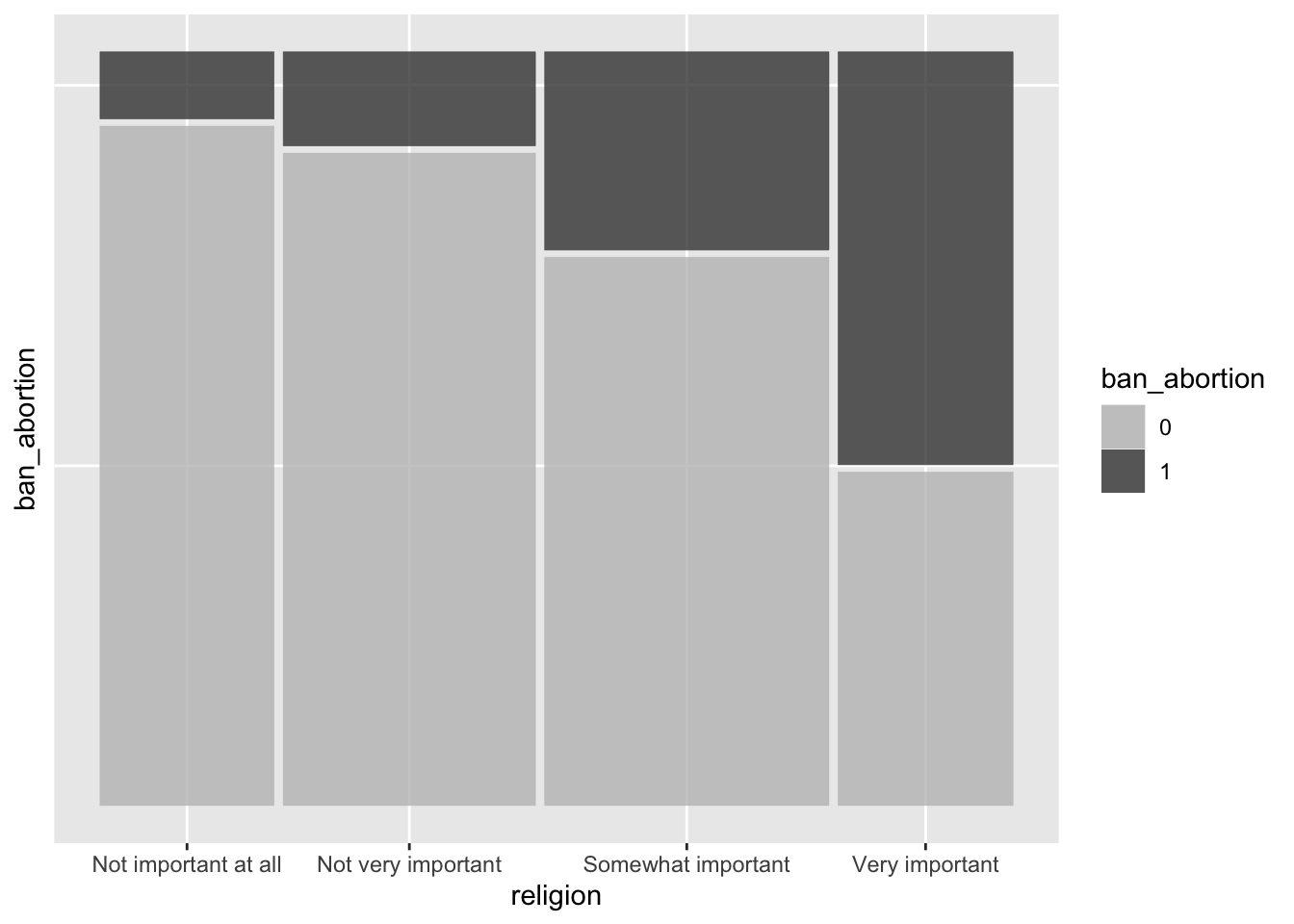
Step 3: Fit linear probability models
Clue
Use lm.
Solution
LM1 <- lm(ban_abortion ~ age, data = ces)
summary(LM1)
Call:
lm(formula = ban_abortion ~ age, data = ces)

Residuals:
    Min      1Q  Median      3Q     Max
-0.2251 -0.2032 -0.1925 -0.1762  0.8294

Coefficients:
             Estimate Std. Error t value Pr(>|t|)
(Intercept) 0.1578475  0.0113846  13.865  < 2e-16 ***
age         0.0007079  0.0002034   3.481 0.000501 ***
---
Signif. codes:  0 '***' 0.001 '**' 0.01 '*' 0.05 '.' 0.1 ' ' 1

Residual standard error: 0.3966 on 13709 degrees of freedom
  (5252 observations deleted due to missingness)
Multiple R-squared:  0.0008831, Adjusted R-squared:  0.0008102
F-statistic: 12.12 on 1 and 13709 DF,  p-value: 0.0005012
LM2 <- lm(ban_abortion ~ age + female + urban + education, data = ces)
summary(LM2)
Call:
lm(formula = ban_abortion ~ age + female + urban + education,
    data = ces)

Residuals:
    Min      1Q  Median      3Q     Max
-0.3502 -0.2075 -0.1838 -0.1512  0.8566

Coefficients:
                   Estimate Std. Error t value Pr(>|t|)
(Intercept)       0.3345742  0.0265301  12.611  < 2e-16 ***
age               0.0001902  0.0002128   0.894 0.371246
female           -0.0474666  0.0070247  -6.757 1.47e-11 ***
urban            -0.0098662  0.0075416  -1.308 0.190816
educationHS      -0.0838340  0.0243895  -3.437 0.000589 ***
educationSome PS -0.1374527  0.0238905  -5.753 8.93e-09 ***
educationCollege -0.1027191  0.0236662  -4.340 1.43e-05 ***
educationBA      -0.1314366  0.0234618  -5.602 2.16e-08 ***
educationMA+     -0.1274048  0.0242395  -5.256 1.49e-07 ***
---
Signif. codes:  0 '***' 0.001 '**' 0.01 '*' 0.05 '.' 0.1 ' ' 1

Residual standard error: 0.3957 on 13518 degrees of freedom
  (5436 observations deleted due to missingness)
Multiple R-squared:  0.008338,  Adjusted R-squared:  0.007751
F-statistic: 14.21 on 8 and 13518 DF,  p-value: < 2.2e-16
The R-squared is very low (0 %). This linear model is not adapted to predict a binary dependent variable such as ban_abortion.
# spot the issue by inspecting residuals
ggplot(data = NULL, aes(x = resid(LM2))) +
  geom_histogram()
`stat_bin()` using `bins = 30`. Pick better value with `binwidth`.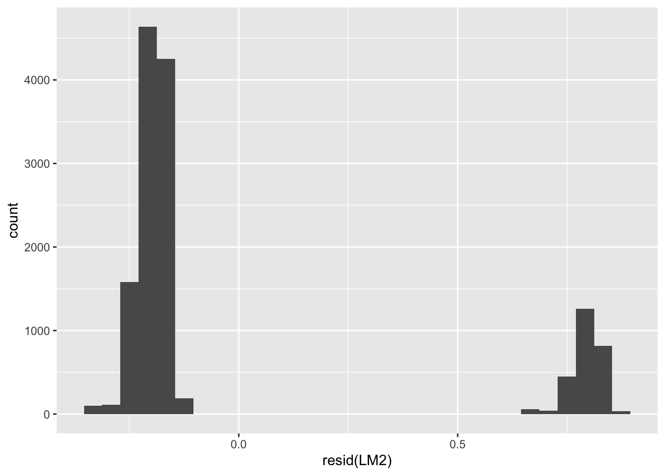
# understand why the residuals are distributed that way
broom::augment(LM2, newdata = ces) %>%
  drop_na(ban_abortion) %>%
  select(respid, ban_abortion, .fitted, .resid) %>%
  sample_n(10)
# A tibble: 10 × 4
respid ban_abortion .fitted .resid
<chr> <dbl> <dbl> <dbl>
1 R_2qCxBVmrOMtCBne 0 0.186 -0.186
2 R_3sBmGjiDJUIzQPx 0 0.213 -0.213
3 R_24kr2fLu95qrwPu 0 0.207 -0.207
4 R_12DsZUpSwANhkzr 0 0.154 -0.154
5 R_3iW68vCTiVlpdTf 0 0.150 -0.150
6 R_1CI5quDlkYPrlxG 1 0.152 0.848
7 R_2fp8oWlkwpOE7AU 0 0.210 -0.210
8 R_RfpLTZnfrys703L 0 0.204 -0.204
9 R_1Q4Ws4mzqrPMpse 0 0.152 -0.152
10 R_VPejiienm7bsrJL 1 0.210 0.790The residuals should have a “normal” / “gaussian” distribution. It is not the case here. Observe the difference between the observed and predicted values of Y and understand why the model is not that good.
Note: To relevel a factor in the predictors when fitting a logistic regression, you can use the relevel function to change the reference level of the factor variable before or during fitting the model:
lm(x ~ y + relevel(b, ref = "3")) Step 4: Fit generalized linear models
Clue
Use glm.
Solution
# 'null model' (intercept-only)
GLM0 <- glm(ban_abortion ~ 1, data = ces, family = binomial(link = "logit"))
summary(GLM0)
Call:
glm(formula = ban_abortion ~ 1, family = binomial(link = "logit"),
    data = ces)

Coefficients:
            Estimate Std. Error z value Pr(>|z|)
(Intercept) -1.41350    0.02153  -65.66   <2e-16 ***
---
Signif. codes:  0 '***' 0.001 '**' 0.01 '*' 0.05 '.' 0.1 ' ' 1

(Dispersion parameter for binomial family taken to be 1)

    Null deviance: 13556  on 13710  degrees of freedom
Residual deviance: 13556  on 13710  degrees of freedom
  (5252 observations deleted due to missingness)
AIC: 13558

Number of Fisher Scoring iterations: 4
# logistic regression model 1
GLM1 <- glm(
ban_abortion ~ age + female + urban + education,
data = ces,
family = binomial(link = "logit")
)
# logistic regression model 2
GLM2 <- glm(
ban_abortion ~ age + female + urban + education + religion,
data = ces,
family = binomial(link = "logit")
)
Clue
\[p = \frac{e^{\alpha + \beta X}}{1 + e^{\alpha + \beta X}}\]
Solution
# reverse the log-odds transformation
exp(coef(GLM0)) / (1 + exp(coef(GLM0)))
(Intercept)
0.1956823 prop.table(table(ces$ban_abortion))
        0         1
0.8043177 0.1956823
Clue
Use ?texreg::screenreg
Solution
# compare results
texreg::screenreg(list(GLM0, GLM1, GLM2))
====================================================================
                            Model 1       Model 2       Model 3
--------------------------------------------------------------------
(Intercept)                    -1.41 ***     -0.67 ***     -0.89 ***
                               (0.02)        (0.15)        (0.20)
age                                           0.00         -0.01 ***
                                             (0.00)        (0.00)
female                                       -0.30 ***     -0.53 ***
                                             (0.04)        (0.05)
urban                                        -0.06         -0.14 *
                                             (0.05)        (0.06)
educationHS                                  -0.42 **      -0.62 ***
                                             (0.14)        (0.17)
educationSome PS                             -0.76 ***     -0.88 ***
                                             (0.13)        (0.17)
educationCollege                             -0.53 ***     -0.63 ***
                                             (0.13)        (0.16)
educationBA                                  -0.72 ***     -0.92 ***
                                             (0.13)        (0.16)
educationMA+                                 -0.69 ***     -0.92 ***
                                             (0.14)        (0.17)
religionNot very important                                  0.44 ***
                                                           (0.10)
religionSomewhat important                                  1.39 ***
                                                           (0.09)
religionVery important                                      2.70 ***
                                                           (0.10)
--------------------------------------------------------------------
AIC                         13558.29      13305.45       8876.42
BIC                         13565.82      13373.07       8961.96
Log Likelihood              -6778.15      -6643.73      -4426.21
Deviance                    13556.29      13287.45       8852.42
Num. obs.                   13711         13527          9214
====================================================================
*** p < 0.001; ** p < 0.01; * p < 0.05
Model 3 (GLM2) minimizes the AIC and BIC indicators. It seems to be the best model here.
Clue
Use ?broom::tidy with the parameter exponentiate = TRUE
Solution
broom::tidy(GLM2, exponentiate = FALSE)# A tibble: 12 × 5
term estimate std.error statistic p.value
<chr> <dbl> <dbl> <dbl> <dbl>
1 (Intercept) -0.888 0.203 -4.37 1.22e- 5
2 age -0.00670 0.00169 -3.97 7.29e- 5
3 female -0.527 0.0549 -9.59 9.13e- 22
4 urban -0.139 0.0577 -2.41 1.61e- 2
5 educationHS -0.619 0.169 -3.67 2.38e- 4
6 educationSome PS -0.879 0.167 -5.26 1.45e- 7
7 educationCollege -0.630 0.163 -3.86 1.14e- 4
8 educationBA -0.921 0.163 -5.65 1.62e- 8
9 educationMA+ -0.922 0.170 -5.42 5.85e- 8
10 religionNot very important 0.438 0.102 4.29 1.76e- 5
11 religionSomewhat important 1.39 0.0936 14.9 2.93e- 50
12 religionVery important 2.70 0.0972 27.7 3.01e-169# exponentiate Model 2 coefficients to read log-odds
broom::tidy(GLM2, exponentiate = TRUE)# A tibble: 12 × 5
term estimate std.error statistic p.value
<chr> <dbl> <dbl> <dbl> <dbl>
1 (Intercept) 0.412 0.203 -4.37 1.22e- 5
2 age 0.993 0.00169 -3.97 7.29e- 5
3 female 0.591 0.0549 -9.59 9.13e- 22
4 urban 0.870 0.0577 -2.41 1.61e- 2
5 educationHS 0.538 0.169 -3.67 2.38e- 4
6 educationSome PS 0.415 0.167 -5.26 1.45e- 7
7 educationCollege 0.532 0.163 -3.86 1.14e- 4
8 educationBA 0.398 0.163 -5.65 1.62e- 8
9 educationMA+ 0.398 0.170 -5.42 5.85e- 8
10 religionNot very important 1.55 0.102 4.29 1.76e- 5
11 religionSomewhat important 4.03 0.0936 14.9 2.93e- 50
12 religionVery important 14.8 0.0972 27.7 3.01e-169# predicted probability of Pr ( ban abortion = Yes )
p <- predict(GLM2, type = "response", newdata = ces)
summary(p) Min. 1st Qu. Median Mean 3rd Qu. Max. NA's
0.046 0.106 0.190 0.249 0.330 0.831 9749 Going further
Prediction success, using p = 0.5 (confusion table)
(t <- table(ces$ban_abortion, p > 0.5, exclude = NULL))
       FALSE TRUE <NA>
  0     6358  566 4104
  1     1506  784  393
  <NA>     0    0 5252
Model accuracy at the 0.5 threshold
100 * sum(diag(t)) / sum(t)[1] 65.35886Another way to obtain and visualize predicted probabilities
ggplot(
  broom::augment(GLM2, newdata = ces, type.predict = "response"),
  aes(y = ban_abortion, x = religion)
) +
  geom_jitter(aes(color = .fitted > 0.5), alpha = 1/3, height = 0.1) +
  scale_y_continuous(breaks = c(0, 0.5, 1), labels = c("0 (N)", 0.5, "1 (Y)"))
Warning: Removed 5252 rows containing missing values or values outside the scale range
(`geom_point()`).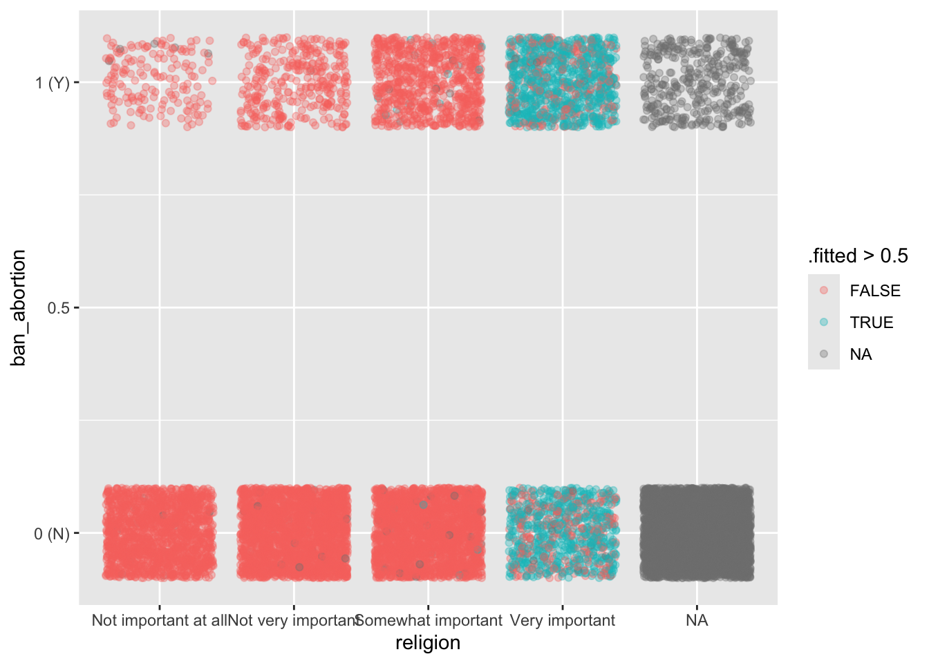
Regression diagnostics (compare to those of linear models).
performance::check_collinearity(GLM2)# Check for Multicollinearity
Low Correlation
Term VIF VIF 95% CI Increased SE Tolerance Tolerance 95% CI
age 1.07 [1.05, 1.10] 1.04 0.93 [0.91, 0.95]
female 1.08 [1.06, 1.11] 1.04 0.92 [0.90, 0.94]
urban 1.03 [1.02, 1.06] 1.02 0.97 [0.94, 0.98]
education 1.08 [1.06, 1.10] 1.04 0.93 [0.91, 0.95]
religion 1.05 [1.03, 1.08] 1.02 0.95 [0.93, 0.97]performance::check_heteroscedasticity(GLM2)This Breusch-Pagan Test currently only works Gaussian models.NULLStep 5: Interact gender and urban residency
GLM3 <- glm(
  ban_abortion ~ age + female * urban + education + religion,
  data = ces,
  family = binomial(link = "logit")
)

GLM4 <- glm(
  ban_abortion ~ age + female:urban + education + religion,
  data = ces,
  family = binomial(link = "logit")
)
texreg::screenreg(list(GLM2, GLM3, GLM4))
====================================================================
                            Model 1       Model 2       Model 3
--------------------------------------------------------------------
(Intercept)                    -0.89 ***     -0.89 ***     -1.15 ***
                               (0.20)        (0.21)        (0.20)
age                            -0.01 ***     -0.01 ***     -0.01 **
                               (0.00)        (0.00)        (0.00)
female                         -0.53 ***     -0.51 ***
                               (0.05)        (0.10)
urban                          -0.14 *       -0.13
                               (0.06)        (0.08)
educationHS                    -0.62 ***     -0.62 ***     -0.65 ***
                               (0.17)        (0.17)        (0.17)
educationSome PS               -0.88 ***     -0.88 ***     -0.88 ***
                               (0.17)        (0.17)        (0.17)
educationCollege               -0.63 ***     -0.63 ***     -0.64 ***
                               (0.16)        (0.16)        (0.16)
educationBA                    -0.92 ***     -0.92 ***     -0.91 ***
                               (0.16)        (0.16)        (0.16)
educationMA+                   -0.92 ***     -0.92 ***     -0.89 ***
                               (0.17)        (0.17)        (0.17)
religionNot very important      0.44 ***      0.44 ***      0.42 ***
                               (0.10)        (0.10)        (0.10)
religionSomewhat important      1.39 ***      1.39 ***      1.37 ***
                               (0.09)        (0.09)        (0.09)
religionVery important          2.70 ***      2.70 ***      2.66 ***
                               (0.10)        (0.10)        (0.10)
female:urban                                 -0.02         -0.46 ***
                                             (0.11)        (0.06)
--------------------------------------------------------------------
AIC                          8876.42       8878.39       8907.61
BIC                          8961.96       8971.06       8986.02
Log Likelihood              -4426.21      -4426.19      -4442.81
Deviance                     8852.42       8852.39       8885.61
Num. obs.                    9214          9214          9214
====================================================================
*** p < 0.001; ** p < 0.01; * p < 0.05
Step 6: plot Predicted probabilities
# predicted probabilities
ggeffects::ggpredict(GLM2, ~ female + education)
# Predicted probabilities of ban_abortion
education: Less than HS
female | Predicted | 95% CI
-------------------------------
0 | 0.20 | 0.15, 0.27
1 | 0.13 | 0.10, 0.18
education: HS
female | Predicted | 95% CI
-------------------------------
0 | 0.12 | 0.10, 0.15
1 | 0.08 | 0.06, 0.09
education: Some PS
female | Predicted | 95% CI
-------------------------------
0 | 0.10 | 0.08, 0.12
1 | 0.06 | 0.05, 0.07
education: College
female | Predicted | 95% CI
-------------------------------
0 | 0.12 | 0.10, 0.14
1 | 0.07 | 0.06, 0.09
education: BA
female | Predicted | 95% CI
-------------------------------
0 | 0.09 | 0.08, 0.11
1 | 0.06 | 0.05, 0.07
education: MA+
female | Predicted | 95% CI
-------------------------------
0 | 0.09 | 0.08, 0.11
1 | 0.06 | 0.05, 0.07
Adjusted for:
* age = 55.91
* urban = 0.69
* religion = Not important at all# average marginal effects (AMEs)
ggeffects::ggeffect(GLM2, terms = ~ female + education)# Predicted probabilities of ban_abortion
education: Less than HS
female | Predicted | 95% CI
-------------------------------
0 | 0.44 | 0.36, 0.51
1 | 0.31 | 0.25, 0.38
education: HS
female | Predicted | 95% CI
-------------------------------
0 | 0.29 | 0.26, 0.33
1 | 0.20 | 0.18, 0.22
education: Some PS
female | Predicted | 95% CI
-------------------------------
0 | 0.24 | 0.22, 0.27
1 | 0.16 | 0.14, 0.18
education: College
female | Predicted | 95% CI
-------------------------------
0 | 0.29 | 0.27, 0.32
1 | 0.20 | 0.18, 0.22
education: BA
female | Predicted | 95% CI
-------------------------------
0 | 0.24 | 0.22, 0.26
1 | 0.15 | 0.14, 0.17
education: MA+
female | Predicted | 95% CI
-------------------------------
0 | 0.24 | 0.21, 0.26
1 | 0.15 | 0.13, 0.18# visualize the AMEs
ggeffects::ggeffect(GLM2, terms = ~ education + religion) %>%
base::plot()Source
Data source: Stephenson, Laura B; Harell, Allison; Rubenson, Daniel; Loewen, Peter John, 2022, “2021 Canadian Election Study (CES)”, doi:10.7910/DVN/XBZHKC, Harvard Dataverse, V1.
More details on the data can be obtained from the Canadian Election Study website.
The example used in the code comes from Andi Fugard’s Using R for Social Research, ch. 9 (“Complex Surveys”), which references Fox and Weinberg as its own data source:
Fox, J. & Weisberg, S. (2019). An R Companion to Applied Regression, 3rd ed., Sage.
R code to generate the ces21-extract dataset
The extract was exported from a Stata session:
use "2021 Canadian Election Study v1.0.dta", clear
gen respid = cps21_ResponseId
gen ban_abortion = (pes21_abort2 < 3) if !mi(pes21_abort2)
gen age = cps21_age
gen female = (cps21_genderid == 2) if cps21_genderid < 3
gen urban = (pes21_rural_urban > 3) if pes21_rural_urban < 6
clonevar religion = cps21_rel_imp if cps21_rel_imp < 5
recode cps21_education ///
    (1/4 = 1 "Less than HS") (5 = 2 "HS") (6 8 = 3 "Some PS") ///
    (7 = 4 "College") (9 = 5 "BA") (10 11 = 6 "MA+") ///
    (else = .), gen(education)

outsheet respid cps21_province cps21_weight_general_restricted ///
    ban_abortion age female urban religion education ///
    if !mi(cps21_weight_general_restricted) ///
    using data/ces21-extract.tsv, replace