repository <- "data"Preparation: Growth forecasts and fiscal consolidation
For Session 10
This exercise focuses on estimating, manipulating and interpreting (simple) linear models. Prior exposure to Keynesian macroeconomics will help, but is not required.
Scenario
You are interning at the Financial Times (FT), under the auspices of Chris Giles.
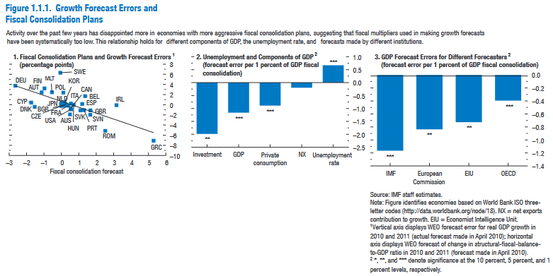
Giles has just released a story titled “Robustness of IMF data scrutinised” (October 12, 2012), in which he tries, and fails, to replicate some of the results published in the World Economic Outlook 2012 report of the International Monetary Fund (IMF).
Giles asks you to independently check that his calculations, which cast some doubt on Box 1.1 of the report (pp. 41–3, “Are We Underestimating Short-Term Fiscal Multipliers?”), are correct.
Instructions
Start by reading all relevant sources (at least those still available…) cited in the scenario above.
Then:
Clue
readxl::read_excel and dplyr::select
Solution
library(readxl)library(tidyverse) # {dplyr}, {ggplot2}, {readxl}, {stringr}, {tidyr}, etc.d <- readxl::read_excel(paste0(repository, "/IMFmultipliers.xlsx"), sheet = 2, skip = 2)New names:
• `` -> `...1`
• `GDP forecast` -> `GDP forecast...2`
• `` -> `...3`
• `` -> `...5`
• `` -> `...6`
• `` -> `...8`
• `` -> `...9`
• `GDP forecast` -> `GDP forecast...10`
• `` -> `...11`
• `` -> `...12`
• `` -> `...13`
• `` -> `...15`d <- d %>%
select(country = `...1`, Dgrowth, Dstruct, DCAPB, cadef = `CA Def`)
Clue
countrycode::countrycode, dplyr::mutate, tidyr::drop_na and dplyr::filter
Solution
# take a look at the variable country
print(d %>% select(country), n = Inf)
# A tibble: 49 × 1
country
<chr>
1 Australia
2 Austria
3 Belgium
4 Canada
5 Cyprus
6 Czech Republic
7 Denmark
8 Finland
9 France
10 Germany
11 Greece
12 Hong Kong SAR
13 Iceland
14 Ireland
15 Israel
16 Italy
17 Japan
18 Korea
19 Luxembourg
20 Malta
21 Netherlands
22 New Zealand
23 Norway
24 Portugal
25 Singapore
26 Slovak Republic
27 Slovenia
28 Spain
29 Sweden
30 Switzerland
31 Taiwan Province of China
32 United Kingdom
33 United States
34 <NA>
35 Albania
36 Bosnia and Herzegovina
37 Bulgaria
38 Croatia
39 Estonia
40 Hungary
41 Kosovo
42 Latvia
43 Lithuania
44 Former Yugoslav Republic of Macedonia
45 Montenegro
46 Poland
47 Romania
48 Serbia
49 Turkey # use countrycode to filter countries
d <- d %>%
mutate(
ccode = countrycode::countrycode(country, "country.name", "genc3c"),
# identify European countries
region = countrycode::countrycode(ccode, "genc3c", "region"),
eu = stringr::str_detect(region, "Europe") | ccode %in% "MLT",
# identify IMF country subset
imf_subset = eu | ccode %in% c("AUS", "CAN", "JPN", "KOR", "USA"),
# identify Chris Giles country subsets
giles_subset1 = !ccode %in% c("NZL", "DEU", "GRC"),
giles_subset2 = !ccode %in% c("DEU", "GRC")
) %>%
# drop empty (gap) row
tidyr::drop_na(country)
# create subsets
d_imf <- d %>% filter(imf_subset)
d_cg1 <- d %>% filter(giles_subset1)
d_cg2 <- d %>% filter(giles_subset2)
Clue
plotting functions, mainly using ggplot2 : ggplot2::geom_point, ggrepel::geom_text_repel, ggplot2::geom_smooth and ggplot2::scale_x_continuous + ggplot2::scale_y_continuous
Solution
ggplot(data = NULL, mapping = aes(y = Dgrowth, x = Dstruct)) +
  # 1. Points and associated labels
  ## IMF subset
  geom_point(data = d_imf, color = "steelblue") +
  ggrepel::geom_text_repel(data = d_imf, aes(label = ccode), color = "steelblue") +
  ## non IMF subset
  geom_point(data = d %>% filter(!imf_subset), color = "darkred") +
  ggrepel::geom_text_repel(data = d %>% filter(!imf_subset), aes(label = ccode), color = "darkred") +
  # 2. Regressions
  ## IMF subset
  geom_smooth(data = d_imf, method = "lm", se = FALSE, color = "steelblue") +
  ## All dataset
  geom_smooth(data = d, method = "lm", se = FALSE, color = "darkred") +
  # 3. Breaks : 1 unit for x, 2 units for y
  scale_x_continuous(breaks = scales::breaks_width(1)) +
  scale_y_continuous(breaks = scales::breaks_width(2))
`geom_smooth()` using formula = 'y ~ x'Warning: Removed 20 rows containing non-finite outside the scale range
(`stat_smooth()`).`geom_smooth()` using formula = 'y ~ x'Warning: Removed 24 rows containing non-finite outside the scale range
(`stat_smooth()`).Warning: Removed 20 rows containing missing values or values outside the scale range
(`geom_point()`).Warning: Removed 20 rows containing missing values or values outside the scale range
(`geom_text_repel()`).Warning: Removed 4 rows containing missing values or values outside the scale range
(`geom_point()`).Warning: Removed 4 rows containing missing values or values outside the scale range
(`geom_text_repel()`).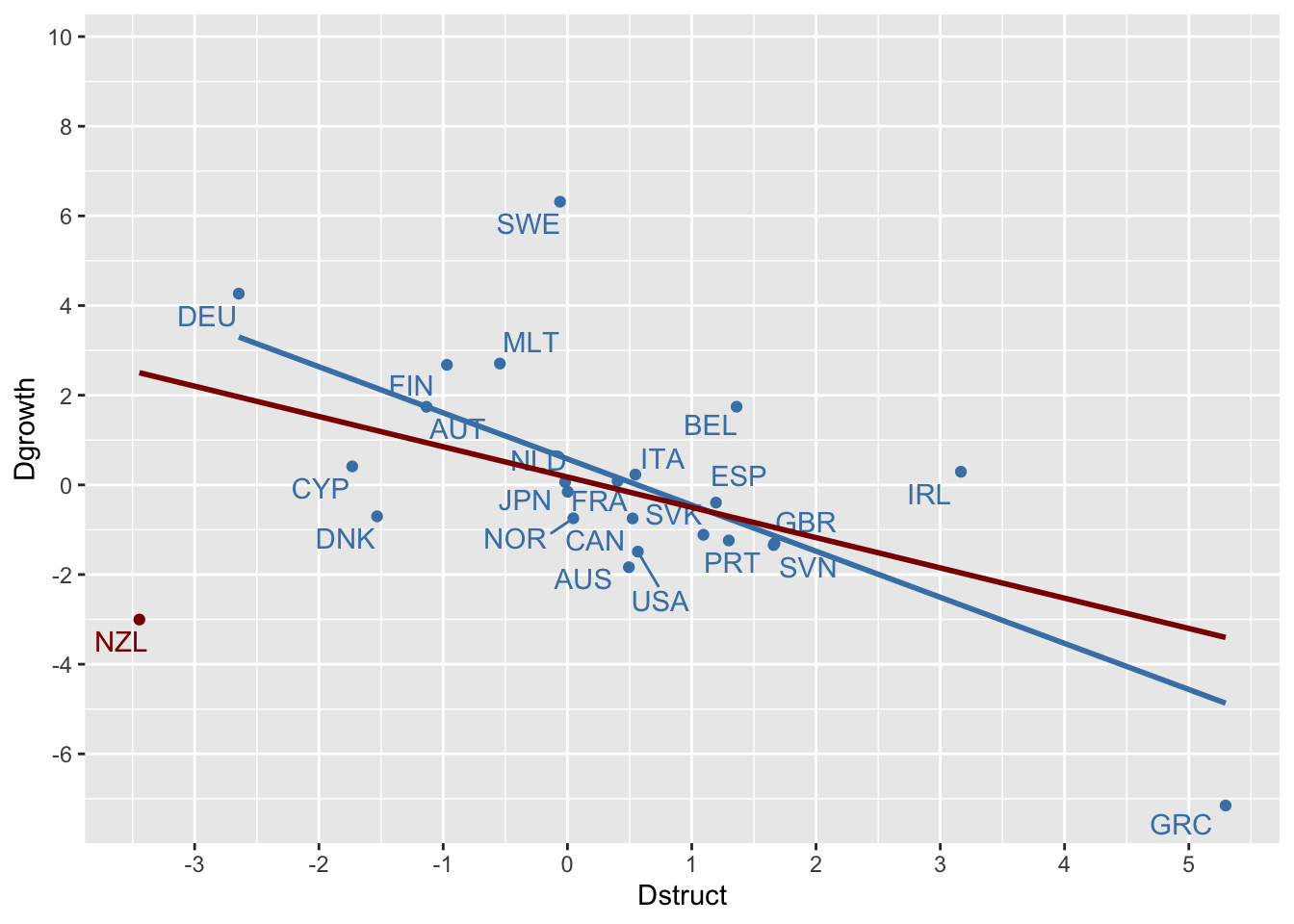
Clue
- Regressions with
lm - Compare models with
texreg::screenreg - Goodness-of-fit (RMSE) with
performance::compare_performance
Solution
#library(broom)
library(performance)
library(texreg)
# regression models
M1 <- lm(Dgrowth ~ Dstruct, data = d_imf)
M2 <- lm(Dgrowth ~ Dstruct, data = d)
M3 <- lm(Dgrowth ~ Dstruct, data = d_cg1)
M4 <- lm(Dgrowth ~ DCAPB, data = d)
M5 <- lm(Dgrowth ~ DCAPB, data = d_cg2)
M6 <- lm(Dgrowth ~ Dstruct + cadef, data = d)
M7 <- lm(Dgrowth ~ Dstruct + cadef, data = d_cg2)
m <- list(M1, M2, M3, M4, M5, M6, M7)
texreg::screenreg(m)
============================================================================
             Model 1    Model 2  Model 3  Model 4  Model 5  Model 6  Model 7
----------------------------------------------------------------------------
(Intercept)   0.58       0.18     0.45     1.32 *   1.13     0.29     0.20
             (0.42)     (0.48)   (0.43)   (0.57)   (0.61)   (0.46)   (0.44)
Dstruct      -1.03 ***  -0.68 *  -0.52                      -0.49    -0.01
             (0.25)     (0.27)   (0.35)                     (0.27)   (0.31)
DCAPB                                     -0.60 *  -0.31
                                          (0.22)   (0.34)
cadef                                                        0.16     0.11
                                                            (0.09)   (0.08)
----------------------------------------------------------------------------
R^2           0.45       0.23     0.10     0.18     0.03     0.33     0.08
Adj. R^2      0.42       0.19     0.06     0.16    -0.00     0.27    -0.02
Num. obs.    23         24       21       35       33       24       22
============================================================================
*** p < 0.001; ** p < 0.01; * p < 0.05
# root mean squared error, as an alternative to R-squared
performance::compare_performance(m) %>%
select(Name, RMSE) %>%
arrange(RMSE)When comparing models, please note that probably not all models were fit
from same data.# Comparison of Model Performance Indices
Name | RMSE
---------------
Model 3 | 1.768
Model 1 | 1.854
Model 7 | 1.866
Model 6 | 2.059
Model 2 | 2.220
Model 4 | 3.034
Model 5 | 3.061The RMSE has to be minimized, thus Model 3 seems to be the best.
The best RMSE are for IMF subset (European Union countries, plus Australia, Canada, Japan, Korea and the United States) and for Giles subset #1 (all countries except New Zealand, Germany and Greece). The worst RMSE are associated with the dataset of all countries and Giles subset #2 (all countries except Germany and Greece).
The IMF databases did not include data for Korea, Hungary, Romania, Bulgaria and Poland and while it did contain data for New Zealand, the country was not included even though Australia was. However, the RMSE are much worst when NZ (obvious outlier) is included. The correlation is much less robust without this outlier.
Solution
# dataset of residuals
data_resid = data.frame(
  value = c(resid(M1),
            resid(M2),
            resid(M3),
            resid(M4),
            resid(M5),
            resid(M6),
            resid(M7)),
  model = c(rep("Model 1", length(resid(M1))),
            rep("Model 2", length(resid(M2))),
            rep("Model 3", length(resid(M3))),
            rep("Model 4", length(resid(M4))),
            rep("Model 5", length(resid(M5))),
            rep("Model 6", length(resid(M6))),
            rep("Model 7", length(resid(M7)))
  )
)

# residuals distributions
  ggplot(data_resid, aes(x = value)) +
  geom_density() +
  # help assessing symmetry
  geom_vline(xintercept = 0, lty = "dashed") +
  facet_wrap(~ model)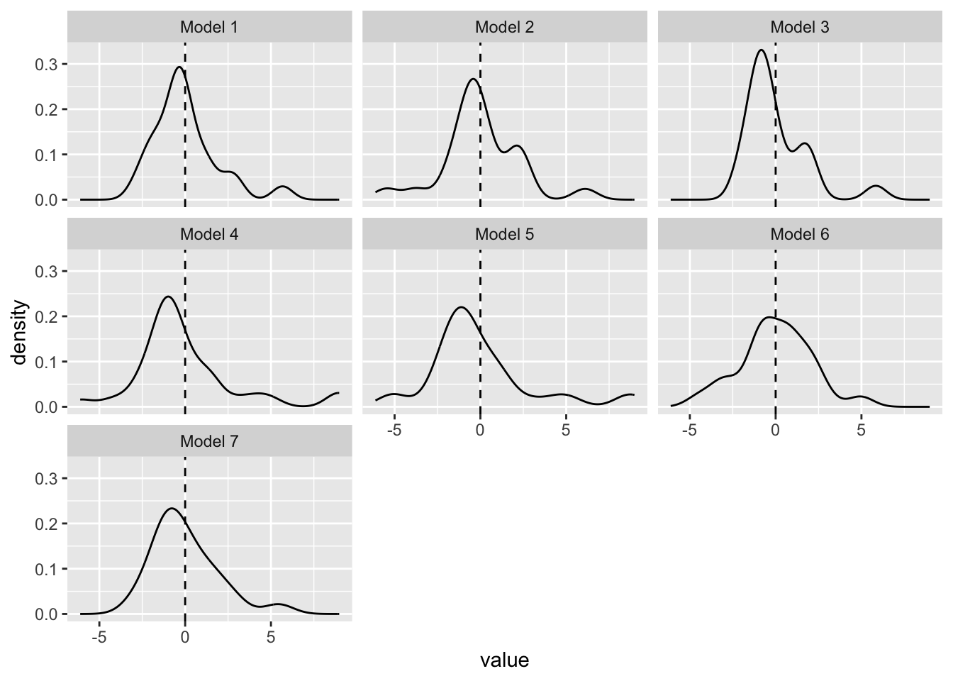
# Advanced coding
purrr::map_dfr(m, ~ tibble::as_tibble_col(resid(.x)), .id = "model") %>%
  mutate(model = str_c("Model ", model))
# quick explainer of how this is coded:
# 1. `map` allows you to apply a function, e.g. `resid`, to a list
map(m, ~ resid(.x))
# 2. you can convert the result of that function to a data frame column
map(m, ~ tibble::as_tibble_col(resid(.x)))
# 3. instead of `map`, use `purrr::map_dfr` to bind all those columns into one
purrr::map_dfr(m, ~ tibble::as_tibble_col(resid(.x)))
# 4. and since you need each series to be identifiable, give them an `.id`
purrr::map_dfr(m, ~ tibble::as_tibble_col(resid(.x)), .id = "model")
Advanced questions [DON’T DO THEM]
Solution
# residuals-versus-fitted values (Model 2)
broom::augment(M2, data = tidyr::drop_na(d, Dgrowth, Dstruct)) %>%
  ggplot(aes(y = .resid, x = .fitted)) +
  geom_hline(yintercept = 0, lty = "dotted") +
  geom_smooth(se = FALSE) +
  geom_text(aes(label = ccode)) +
  theme_linedraw()
`geom_smooth()` using method = 'loess' and formula = 'y ~ x'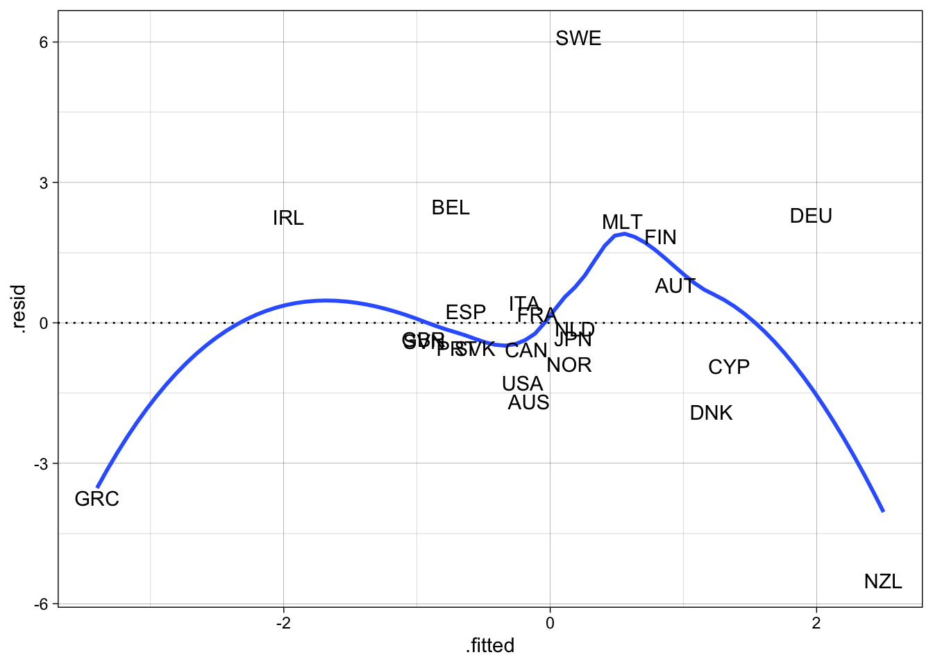
Solution
# Cook's distance
broom::augment(M2, data = tidyr::drop_na(d, Dgrowth, Dstruct)) %>%
  filter(.cooksd > 1) %>%
  pull(country)
[1] "Greece" "New Zealand"# standardized residuals
broom::augment(M2, data = tidyr::drop_na(d, Dgrowth, Dstruct)) %>%
filter(abs(.std.resid) > 2) %>%
pull(country)[1] "Greece" "New Zealand" "Sweden" # standardized residuals, visually
broom::augment(M2, data = tidyr::drop_na(d, Dgrowth, Dstruct)) %>%
ggplot(aes(y = .std.resid, x = .fitted)) +
geom_rug() +
geom_hline(yintercept = c(-2, 0, 2), lty = "dotted") +
geom_point(aes(color = abs(.std.resid)), size = 15, alpha = 3/4) +
geom_text(aes(label = ccode)) +
scale_color_binned(low = "white", high = "tomato") +
theme_linedraw()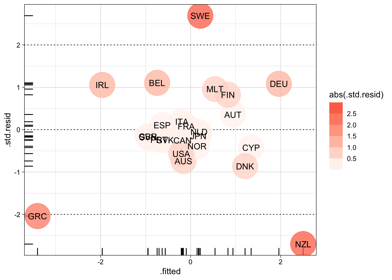
Solution
repository <- "data"# replicate IMF effect size
imf <- readr::read_csv(paste0(repository,"/boxfig1_1_1.csv"), skip = 5) %>%
select(country = `...1`, growth = y, fiscal = `Fiscal consolidation forecast`)New names:
Rows: 28 Columns: 10
── Column specification
──────────────────────────────────────────────────────── Delimiter: "," chr
(4): ...1, Investment, ...8, IMF dbl (4): y, Fiscal consolidation forecast,
-1.987, -1.166122 lgl (2): ...4, ...5
ℹ Use `spec()` to retrieve the full column specification for this data. ℹ
Specify the column types or set `show_col_types = FALSE` to quiet this message.
• `` -> `...1`
• `` -> `...4`
• `` -> `...5`
• `` -> `...8`
Solution
# published coefficient of -1.16
coef(lm(growth ~ fiscal, data = imf))[ "fiscal" ]
fiscal
-1.164258 Source
The data in this folder come from a blog post by Chris Giles that seems not available online anymore:
Chris Giles, “Has the IMF proved multipliers are really large? (wonkish),” Money Supply, 12 October 2012.
However, an archived (and incomplete) version of the relevant blog post can be found at the Internet Archive.
Economics is the science of thinking in terms of models joined to the art of choosing models that are relevant to the contemporary world.
— John Maynard Keynes
To allow the market mechanism to be sole director of the fate of human beings and their natural environment, indeed, even of the amount and use of purchasing power, would result in the demolition of society.
— Karl Polanyi