Exercise 1: Maps of road accidents

Session 11

Authors

Kim Antunez, Etienne Côme

The Etalab database of French road traffic injury accidents for a given year is divided into 4 sections, each represented by a CSV file:

The CARACTERISTIQUES (CHARACTERISTICS) section that describes the general circumstances of the accident.
The LIEUX (LOCATIONS) section that describes the main location of the accident, even if it occurred at an intersection.
The involved VEHICULES (VEHICLES) section.
The involved USAGERS (USERS) section.

Download datasets on your computer

Download the different datasets here:

Different copies are downloaded at different links:

usagers-2021.csv
carcteristiques-2021.csv [be careful of the typo (carc instead of caract)]
lieux-2021.csv
vehicules-2021.csv

You’ll also need different map layers :

Step 1: Load data and install useful packages

library(tidyverse) # {dplyr}, {ggplot2}, {readxl}, {stringr}, {tidyr}, etc.

library(sf)

Linking to GEOS 3.11.0, GDAL 3.5.3, PROJ 9.1.0; sf_use_s2() is TRUE

library(RColorBrewer)
library(mapview)

repository <- "data"

users <- read.csv2(paste0(repository, "/usagers-2021.csv"))

characteristics <- read.csv2(paste0(repository, "/carcteristiques-2021.csv"))

place <- read.csv2(paste0(repository, "/lieux-2021.csv"))

vehicles <- read.csv2(paste0(repository, "/vehicules-2021.csv"))

Step 2: Manipulate `sf` objects

Question 1

Join the 4 datasets and focus on accidents in Paris (2 first digits of com = 75).

Clue

See ?dplyr::left_join ?dplyr::filter and substr.

Solution

accidents.2021.paris <- users %>%
  select(Num_Acc,id_vehicule,grav,sexe,an_nais) %>%
  left_join(characteristics %>%  select(Num_Acc, lat, long, com, int, lum)) %>%
  left_join( place %>% select(Num_Acc,voie,catr)) %>%
  left_join(vehicles %>% select(Num_Acc,id_vehicule,catv)) %>%
  filter(substr(com,1,2)==75)

Joining with `by = join_by(Num_Acc)`
Joining with `by = join_by(Num_Acc)`
Joining with `by = join_by(Num_Acc, id_vehicule)`

Question 2

Transform the dataset into a sf geographical object (default projection : 4226) and reproject it in Lambert-93 projection (2154)

Clue

sf::st_as_sf with parameters coords and crs.

Solution

accidents.2021.paris <- st_as_sf(accidents.2021.paris,
                                 coords = c("long", "lat"),
                                 crs = 4226) %>% 
  st_transform(2154)

Question 3

Import the ‘iris.75.shp’ iris¹ map of Paris.

Clue

Use sf::st_read().

Solution

library(sf)
iris.75 <- st_read(paste0(repository, "/iris_75.gpkg"), quiet = TRUE,
                   stringsAsFactors = F)

Question 4

Display the map of Paris using the instruction plot(iris.75). What do you notice?

Solution

plot(iris.75)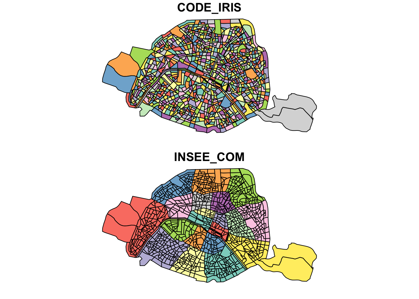

We notice that R makes several graphs: one for each variable contained in the sf object.

Question 5

What is the purpose of the function sf::st_geometry()? What solution do you propose to the previous problem?

Solution

sf::st_geometry() is used to isolate the information contained in the geometry column of the sf object. This allows other variables to be set aside and only one displayed.

plot(st_geometry(iris.75))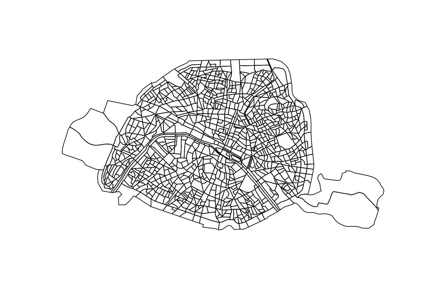

Question 6

Display a map of accidents in Paris simply by using the plot function.

Clue

Use sf::st_geometry(). You can also customize the map using different plot function parameters: bg, col, lwd, border, pch, cex…

Solution

plot(st_geometry(iris.75), bg = "cornsilk", col = "lightblue", 
     border = "white", lwd = .5)
plot(st_geometry(accidents.2021.paris), col = "red", pch = 20, cex = .2, add=TRUE)
title("Accidents in Paris")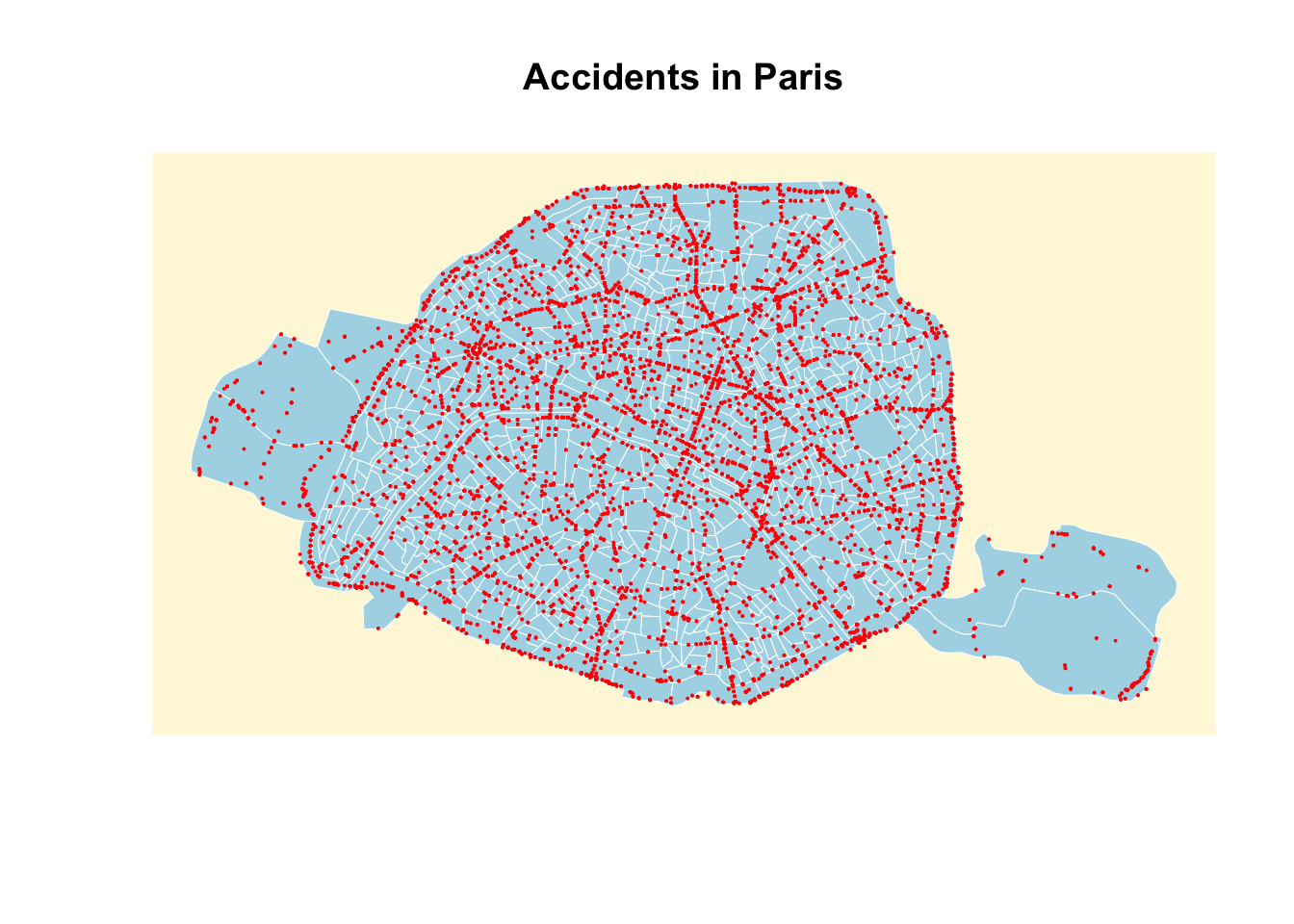

Question 7

Perform at least one of the following geomatic processes:

Create a polygon with the outline of Paris by aggregating the irises of Paris (simple union)
Create a 1km buffer zone around it
Extract iris centroids
Calculate distances between iris centroids
Calculate Voronoi polygons around iris centroids

Display the various map layers created.

Clue

Use st_union, st_buffer, st_voronoi, st_collection_extract, st_interection, st_join and st_centroid.

Solution

# 1. Aggregated map of Paris
iris.75.u <- st_union(iris.75)
# 2. Buffer zone
iris.75.b <- st_buffer(x = iris.75.u, dist = 1000)
# 3. Centroids
iris.75.c <- st_centroid(iris.75)

Warning: st_centroid assumes attributes are constant over geometries

# 4. Distance between centroids
mat <- st_distance(x=iris.75.c, y=iris.75.c)
# 5. Voronoï polygons around centroids
iris.75.v <- st_collection_extract(st_voronoi(x = st_union(iris.75.c)))
iris.75.v <- st_intersection(iris.75.v,iris.75.u)

# Plot maps
plot(st_geometry(iris.75.b), lwd=2, border ="red",col=NA)
plot(st_geometry(iris.75),  ltw=5, col="#999999", add = TRUE)
plot(st_geometry(iris.75.u), border="blue", ltw=5, col=NA, add = TRUE)
plot(st_geometry(iris.75.c), pch = 20, cex = .2,col="red", add = TRUE)
plot(st_geometry(iris.75.v),  ltw=5, col=NA,border="blue", add = TRUE)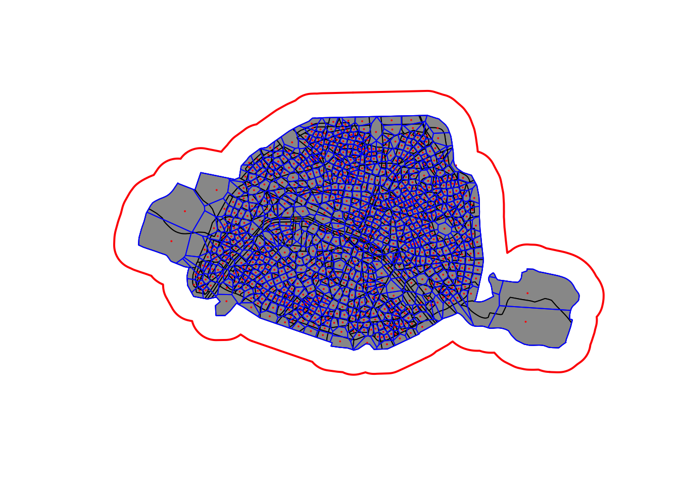

Question 8

Create an ‘accidents.2021.paris.iris’ map layer of iris that counts the number of people involved in accidents per iris, as well as the number of people involved in accidents but not injured.

Keep the Paris arrondissement code in this map layer.

Information

The ‘iris.75’ map layer contains a 5-digit code in its INSEE_COM variable, corresponding to the arrondissement code.

Documentation for the grav variable: Severity of user injury, accident victims are classified into three categories of victims plus the uninjured:

1: Uninjured
2 : Killed
3 : Hospitalized
4 : Slightly injured

Clue

Use sf::st_join() (spatial join) and also functions from the classic dplyr package:

dplyr::select
dplyr::group_by
dplyr::summarise
dplyr::left_join`.

These functions also work with sf objects.

Solution

library(dplyr)
# Spatial join ?st_join with ?st_intersects predicates
accidents.2021.paris.iris <- iris.75  %>%  st_join(accidents.2021.paris,
                                                join = st_intersects)
str(accidents.2021.paris.iris)

Classes 'sf' and 'data.frame':  11235 obs. of  14 variables:
 $ CODE_IRIS  : chr  "751197316" "751197316" "751197316" "751197316" ...
 $ INSEE_COM  : chr  "75119" "75119" "75119" "75119" ...
 $ Num_Acc    : num  2.02e+11 2.02e+11 2.02e+11 2.02e+11 2.02e+11 ...
 $ id_vehicule: chr  "195 100" "195 101" "147 415" "147 415" ...
 $ grav       : int  4 1 1 4 4 1 4 1 4 1 ...
 $ sexe       : int  1 1 -1 2 2 1 1 1 1 1 ...
 $ an_nais    : int  1996 1947 NA 2016 1965 1982 1952 1981 1990 1986 ...
 $ com        : chr  "75119" "75119" "75119" "75119" ...
 $ int        : int  2 2 1 1 1 1 2 2 3 3 ...
 $ lum        : int  1 1 1 1 1 1 1 1 1 1 ...
 $ voie       : chr  "AVENUE DE FLANDRE" "AVENUE DE FLANDRE" "RUE ARCHEREAU" "RUE ARCHEREAU" ...
 $ catr       : int  4 4 4 4 4 4 4 4 4 4 ...
 $ catv       : int  32 7 7 7 1 1 31 14 30 7 ...
 $ geom       :sfc_MULTIPOLYGON of length 11235; first list element: List of 1
  ..$ :List of 1
  .. ..$ : num [1:23, 1:2] 653971 653973 653986 653994 653996 ...
  ..- attr(*, "class")= chr [1:3] "XY" "MULTIPOLYGON" "sfg"
 - attr(*, "sf_column")= chr "geom"
 - attr(*, "agr")= Factor w/ 3 levels "constant","aggregate",..: NA NA NA NA NA NA NA NA NA NA ...
  ..- attr(*, "names")= chr [1:13] "CODE_IRIS" "INSEE_COM" "Num_Acc" "id_vehicule" ...

# Aggregate by CODE_IRIS
accidents.2021.paris.iris <- accidents.2021.paris.iris %>% 
  # To speed up processing: IRIS geometry can be deleted
  # geometry before aggregation and add it later
  st_drop_geometry() %>%
  group_by(CODE_IRIS) %>% 
  summarise(nbacc=n(), nbaccnb =  sum(grav==1)) %>%
  # We put geometry back
  left_join(iris.75 %>% select(CODE_IRIS, INSEE_COM)) %>%
  st_as_sf()

Joining with `by = join_by(CODE_IRIS)`

head(accidents.2021.paris.iris)

Simple feature collection with 6 features and 4 fields
Geometry type: MULTIPOLYGON
Dimension:     XY
Bounding box:  xmin: 650181.1 ymin: 6861761 xmax: 652179 ymax: 6863138
Projected CRS: RGF93 v1 / Lambert-93
# A tibble: 6 × 5
  CODE_IRIS nbacc nbaccnb INSEE_COM                                         geom
  <chr>     <int>   <int> <chr>                               <MULTIPOLYGON [m]>
1 751010101    21       9 75101     (((652130.3 6862122, 652126.1 6862116, 6521…
2 751010102     3       2 75101     (((651807.7 6861881, 651668.7 6862071, 6516…
3 751010103     8       5 75101     (((651639.9 6862522, 651666.9 6862508, 6517…
4 751010104    31      11 75101     (((651134.9 6862419, 650895 6862502, 650854…
5 751010105    14       5 75101     (((650850.3 6862538, 650849.7 6862532, 6508…
6 751010199    21      10 75101     (((650833.2 6862444, 650696 6862519, 650544…

Question 9

Use the ‘accidents.2021.paris.iris’ layer, to create a new aggregated map layer called ‘accidents.2021.paris.arr’ which corresponds to the arrondissements of Paris.

Keep information on the number of people involved in accidents and the number of uninjured accident victims in each arrondissement in this new layer.

Solution

library(dplyr)
accidents.2021.paris.arr <- accidents.2021.paris.iris %>%
  group_by(INSEE_COM) %>%
  summarize(nbacc = sum(nbacc, na.rm=TRUE),
            nbaccnb = sum(nbaccnb, na.rm=TRUE)) 
head(accidents.2021.paris.arr)

Simple feature collection with 6 features and 3 fields
Geometry type: POLYGON
Dimension:     XY
Bounding box:  xmin: 649855.9 ymin: 6859834 xmax: 653707.7 ymax: 6863752
Projected CRS: RGF93 v1 / Lambert-93
# A tibble: 6 × 4
  INSEE_COM nbacc nbaccnb                                                   geom
  <chr>     <int>   <int>                                          <POLYGON [m]>
1 75101       242     103 ((650257 6862732, 650181.1 6862768, 650208.6 6862824,…
2 75102       160      82 ((651769.9 6863020, 651741.2 6863031, 651701 6863047,…
3 75103       186      84 ((652805.5 6862427, 652773.9 6862443, 652688.9 686248…
4 75104       302     125 ((652705.9 6861376, 652544.5 6861441, 652420.3 686148…
5 75105       225     104 ((652395.6 6859839, 652364.6 6859842, 652225.6 685986…
6 75106       151      70 ((650807.6 6860419, 650795.2 6860425, 650752.3 686044…

plot(st_geometry(accidents.2021.paris.iris),
     col = "ivory3", border = "ivory1")
plot(st_geometry(accidents.2021.paris.arr),
     col = NA, border = "ivory4", lwd = 2, add = TRUE)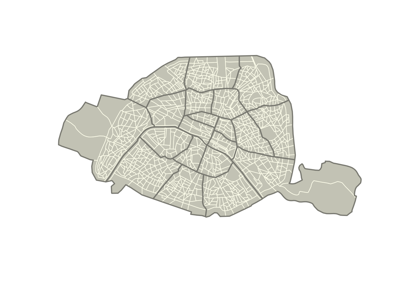

Step 3 : Interactive maps

We’re now going to use mapview to explore road accidents in Paris in 2021.

Question 10

Load the ‘accidents.2021.paris’ database and display the positions of 11,897 accident victims in Paris in 2021 using the mapview package. Try using different parameters to customize your map. Color points according to the severity of accidents.

Information

For example, you can use the parameters col.regions, label, color, legend, layer.name, homebutton, lwd, alpha, zcol … of the mapview package to reproduce the map below.

Solution

library(mapview)
library(sf)

m <- mapview(accidents.2021.paris %>%
          mutate(grav_f = factor(grav,
                         levels = c(2,3,4,1),
                         labels = c("Killed", "Hospitalized",
                                    "Slightly injured", "Uninjured")
                         )),
        col.regions = c("darkred","red","orange","darkgreen"),
        label = accidents.2021.paris$Num_Acc, 
        color = "white", legend = TRUE,
        zcol="grav_f", alpha=0.9,
        layer.name = "Gravite",
        homebutton = FALSE, lwd = 0.2)

Note: only 100 points are shown here to lighten the .html file.

Step 4: Maps with `ggplot2`

We want to create a map of the arrondissements of Paris that combines the number of people involved in accidents and the proportion of those who were not injured.

Question 11

Prepare the data for the card using the following steps:

Load the background map ‘com75_shp’ (which contains the number of accident victims, total and uninjured, in each borough) and create a variable called prop_uninjured which corresponds to the share of uninjured people among accident victims in each borough.
Create a vector of quartiles of the prop_uninjured variable.
Create the color vector corresponding to the number of classes defined earlier.
Add a variable called typo to ‘com.75’ which indicates the rounding class according to the discretization contained in bks for the variable prop_uninjured.

Clue

To create bks and cols, use the quantile and RColorBrewer::brewer.pal functions. To create the typo variable, you can use the cut function with parameters digit.lab = 2 and include.lowest = TRUE.

Solution

library(sf)
# 1. Import dataset and Create the variable prop_uninjured
com.75 <- st_read(paste0(repository, "/com_75.gpkg"), quiet = TRUE)
com.75$prop_uninjured <- 100 * com.75$nbaccnb / com.75$nbacc

# 2. Define breaks with quantiles
bks <- quantile(com.75$prop_uninjured, na.rm = TRUE, probs=seq(0,1,0.25))

# 3. Define color palette
library(RColorBrewer)
cols <- brewer.pal(length(bks)-1,"Greens")

# 4. Variable typo
library(dplyr)
com.75 <- com.75 %>%
  mutate(typo = cut(prop_uninjured,
                    breaks = bks,
                    labels = paste0(
                      round(bks[1:(length(bks)-1)]),
                      " à ",round(bks[2:length(bks)])
                      ),
                    include.lowest = TRUE))

Question 12

Using the ggplot2 package, create a map containing the prop_uninjured variable in choropleth and the nbacc variable in proportional circles.

Solution

library(ggplot2)

map_ggplot <- ggplot() +
  geom_sf(data = com.75, aes(fill = typo), colour = "grey80") +
  scale_fill_manual(name = "Percentage of non-injured\nroad accident victims (%)",
                    values = cols) +
  geom_sf(data = com.75 %>%  st_centroid(),
          aes(size = nbacc), fill = "#f5f5f5", color = "grey20", shape = 21, 
          stroke = 1, alpha = 0.8, show.legend = "point") +
  scale_size_area(max_size = 12, name = "Number of\naccidented people") +
  coord_sf(crs = 2154, datum = NA,
           xlim = st_bbox(com.75)[c(1,3)],
           ylim = st_bbox(com.75)[c(2,4)]) +
  theme_minimal() +
  theme(panel.background = element_rect(fill = "cornsilk", color = NA), 
        legend.position = "bottom", plot.background = element_rect(fill = "cornsilk",color=NA)) +
  labs(title = "Road accidents in Paris in 2021",
       caption = "BAAC 2021 dataset, ONISR\nantuki & comeetie, 2023") +
  guides(size = guide_legend(label.position = "bottom", title.position = "top",
                             override.aes = list(alpha = 1, color = "#ffffff")),
         fill = guide_legend(label.position = "bottom", title.position = "top"))

Warning: st_centroid assumes attributes are constant over geometries

plot(map_ggplot)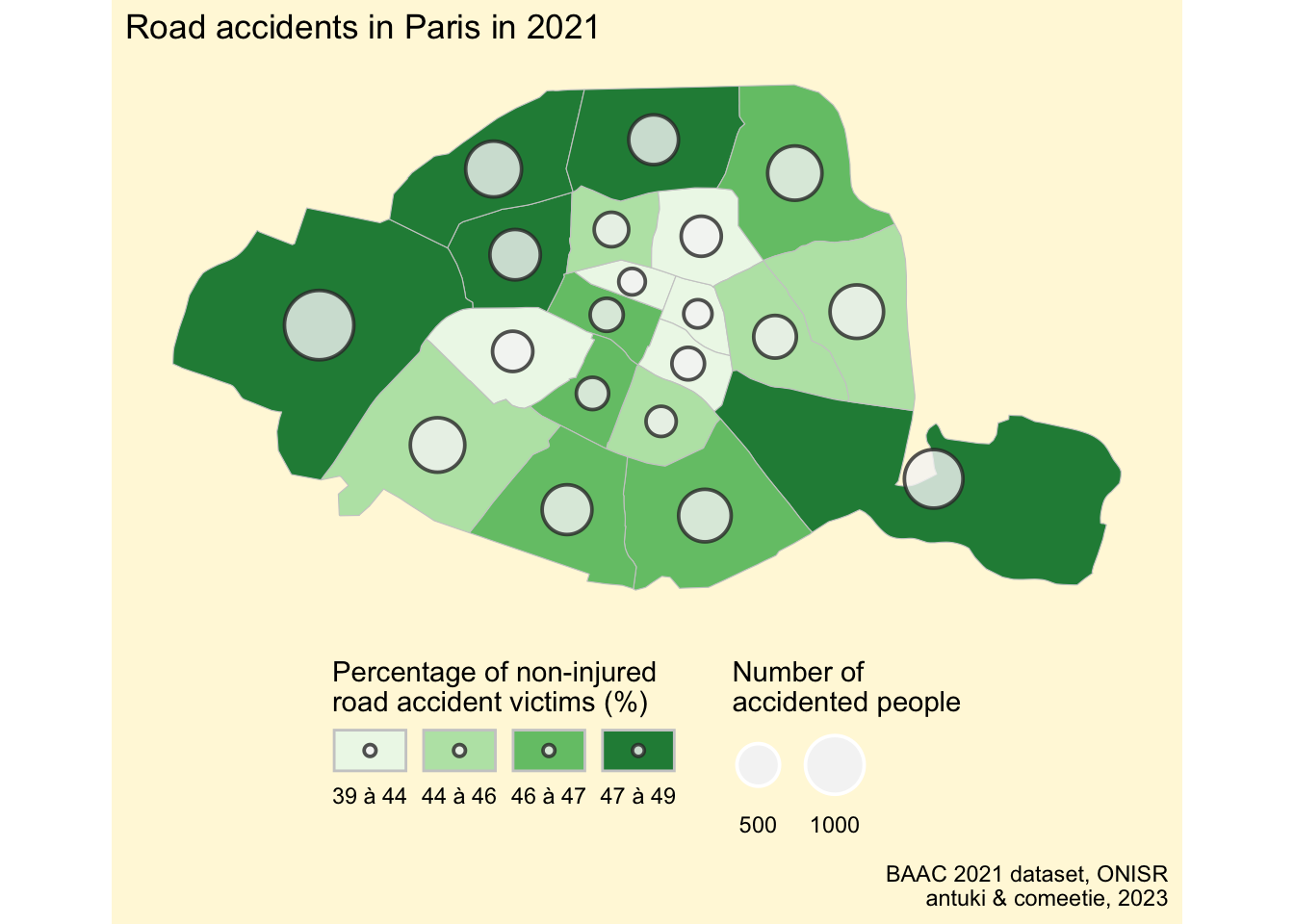

Question 13 [OPTIONAL]

Create the same map with the mapsf package.

Solution

library(mapsf)
mf_theme("default",cex=0.9,mar=c(0,0,1.2,0),bg="ivory")
#mf_init(x = com.75, theme = "ink", expandBB = c(0, 0, 0, .15))
mf_map(
  x = com.75,
  var = "prop_uninjured",
  type = "choro",
  border = "grey80",
  lwd = 0.1,
  leg_pos = c("topright"),
  leg_title = c("Percentage of non-injured\nroad accident victims (%)"),
  breaks = "quantile",
  nbreaks = 4,
  pal = "Greens",
  leg_val_rnd = 0,
  leg_frame = TRUE
)
mf_map(
  x = com.75 %>%  st_centroid(),
  var = "nbacc",
  type = "prop",
  border = "grey20",
  lwd = 0.1,
  leg_pos = c("right"),
  leg_title = c("Number of\naccidented people"),
  col = "#f5f5f5",
  leg_val_rnd = 0,
  leg_frame = TRUE
)
mf_layout(
  title = "Road accidents in Paris in 2021",
  credits = "BAAC 2021 dataset, ONISR\nantuki & comeetie, 2023",
  frame = TRUE)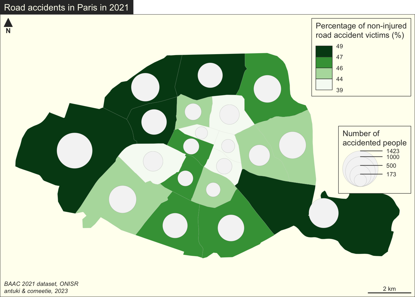

Footnotes

The iris is an Insee statistical zoning system whose acronym stands for “Ilots Regroupés pour l’Information Statistique”. Their size is 2000 inhabitants per unit.↩︎

Download datasets on your computer

Step 1: Load data and install useful packages

Step 2: Manipulate sf objects

Step 3 : Interactive maps

Step 4: Maps with ggplot2

Footnotes

Step 2: Manipulate `sf` objects

Step 4: Maps with `ggplot2`