repository <- "data"Exam 3: Personal R Coding and Reflective Analysis on Skill Acquisition in Data Science
For May the 7th
In this third exam, you will first continue to explore a real-world dataset containing information about road traffic accidents in France in 2022 (Part 1), but this time by yourself and without your group. Then, you will focus on reflecting upon what you did over the course of the semester in this course, and what you make out of it at that stage (Part 2).
This is a graded exercise, to be completed individually and not in groups. Make sure to adhere to all ethical and academic integrity standards.
Part 1: R [10 points]
Download datasets
The Etalab database of French road traffic injury accidents for a given year is divided into 4 sections, each represented by a CSV file:
- The CARACTERISTIQUES (CHARACTERISTICS) section that describes the general circumstances of the accident.
- The LIEUX (LOCATIONS) section that describes the main location of the accident, even if it occurred at an intersection.
- The involved VEHICULES (VEHICLES) section.
- The involved USAGERS (USERS) section.
Download the copies of the two datasets:
usagers-2022.csvcarcteristiques-2022.csv[be careful of the typo (carc instead of caract)]
Then, load the required packages and the datasets into R, exactly as you did for exam 1 and 2 before.
Solution
library(tidyverse) # of simply {dplyr}, {readr}, {ggplot2}.users <- readr::read_delim(paste0(repository, "/usagers-2022.csv"),
show_col_types = FALSE, delim = ";")
characteristics <- readr::read_delim(paste0(repository, "/carcteristiques-2022.csv"), show_col_types = FALSE, delim = ";")full_joined <-
full_join(users %>% rename(Accident_Id = Num_Acc),
characteristics,
by="Accident_Id")
Question 2
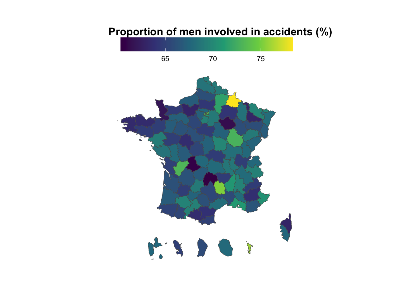
Using a map layer that can be downloaded here, can you draw the following map with the proportion of male involved in accidents for each French “départements” of France.
Solution
library(sf)
geo <- sf::st_read(paste0(repository, "/departements.gpkg"), quiet = TRUE)

data_to_plot <- full_joined %>%
  mutate(sexe = ifelse(sexe==" -1", NA, sexe)) %>%
  mutate(sexe = factor(sexe, levels=c(1,2), labels=c("Male","Female"))) %>%
  group_by(dep, sexe) %>%
  count() %>%
  tidyr::pivot_wider(names_from="sexe", values_from="n") %>%
  mutate(prop_of_men_involved_in_acc = 100 * Male / (Female+Male)) %>%
  right_join(geo, by=c("dep"="DEP")) %>%
  st_as_sf()

ggplot(data_to_plot, aes(fill = prop_of_men_involved_in_acc)) +
  geom_sf() +
  scale_fill_viridis_c("") +
  theme_void() +
   theme(
     legend.position = "top",
     legend.key.width = unit(1.5, "cm"),
     plot.title = element_text(face = "bold"),
     plot.margin = margin(1 ,1 , 1, 1, "cm")
   ) +
  labs(title = "Proportion of men involved in accidents (%)")
Solution
Many answers were possible for this open question. Below for example is the proposal (slightly reworked) from a student.
Do lightning conditions in the night influence the severity of an accident ?
I first clean my dataset so as to only keep the relevant information for this question I call this new dataset light_severity
light_severity <- full_joined %>%
  dplyr::select(Accident_Id, lum, grav)
Now that I have this new dataset, I finish cleaning it by recoding missing variables
print(unique(light_severity$lum))[1] 1 5 3 2 4 NAprint(unique(light_severity$grav))[1] "3" "1" "4" "2" " -1"The “lum” missing values are already coded NA, but not the “grav” missing values which are coded ” -1” I trim the data (remove the ” ” before “-1” ) and then recode with NAs.
light_severity$grav <- trimws(light_severity$grav)
light_severity$grav[light_severity$grav == -1] <- NA
print(unique(light_severity$grav))
[1] "3" "1" "4" "2" NA I only keep the night accidents for my analysis, and I group together “public lighting off” (4) and “no public lighting” (3). For readability, I relabel the different factors.
light_severity <- light_severity %>%
  filter(lum %in% c("3", "4", "5"))

light_severity <- light_severity %>%
  mutate(lum = ifelse(lum == "4", "3", lum))

light_severity <- light_severity %>%
  mutate(grav = case_when(
    grav == "1" ~ "unhurt",
    grav == "2" ~ "killed",
    grav == "3" ~ "hospitalized injury",
    grav == "4" ~ "slight injury"
  ),
  lum = case_when(
    lum == "3" ~ "no public lighting",
    lum == "5" ~ "public lighting on"
  ))
I make a table with counts, and then another table with percentages.
light_severity_table <- table(light_severity$grav, light_severity$lum)
print(light_severity_table)
                      no public lighting public lighting on
  hospitalized injury               3132               2329
  killed                             945                347
  slight injury                     5166               8610
  unhurt                            4968               8532
light_severity_percentage <- prop.table(light_severity_table, margin = 1) * 100 # Percentage by row
print(light_severity_percentage)
                      no public lighting public lighting on
  hospitalized injury           57.35213           42.64787
  killed                        73.14241           26.85759
  slight injury                 37.50000           62.50000
  unhurt                        36.80000           63.20000
I make a bar plot to illustrate my table.
# I first convert the percentage table to a data frame
light_severity_data <- as.data.frame(light_severity_percentage)

# Plot the bar chart
ggplot(light_severity_data, aes(x = factor(Var1), y = Freq, fill = Var2)) +
  geom_bar(stat = "identity", position = "dodge") +
  labs(x = "Severity", y = "Percentage", fill = "Lighting") +
  ggtitle("Accident severity by lighting condition at night") +
  scale_fill_manual(values = c("#005a8a", "#ffee58")) + # Set custom colors for bars
  theme_minimal()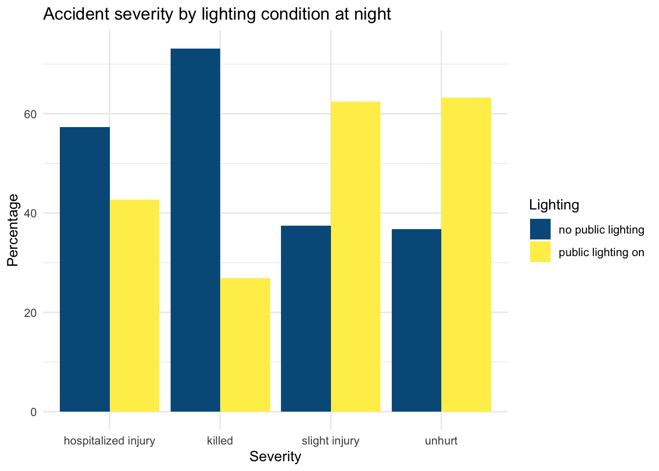
Looking at our plotted bar, we can see that the presence or absence of lighting at night seems to have an impact on the severity of the accident. Unhurt accidents and accidents with slight injuries respectively happen 63.2% and 62.5% of the time with public lighting on. On the other hand, accidents at night where someone gets killed happen 73.1% of the time in places with no public lighting. For hospitalised injuries,this happens 57.4% of the time in places with no public light.
Now I test the significance of my results with a chi-squared test:
chisq_test <- chisq.test(light_severity_table)
print(chisq_test)
    Pearson's Chi-squared test

data:  light_severity_table
X-squared = 1308.4, df = 3, p-value < 2.2e-16
The p-value is less than the significance level of 0.05, which means that we can reject the null hypothesis. Therefore, we can assume with confidence that there is a significant association between accident severity and lighting conditions at night.
KIM : OBSERVED AND THEORETICAL RESIDUALS
chisq_test$observed # this is what you observe in your data
                      no public lighting public lighting on
  hospitalized injury               3132               2329
  killed                             945                347
  slight injury                     5166               8610
unhurt 4968 8532chisq_test$expected # this is what it would look like at random
                      no public lighting public lighting on
  hospitalized injury          2280.5922          3180.4078
  killed                        539.5578           752.4422
  slight injury                5753.0558          8022.9442
unhurt 5637.7942 7862.2058chisq_test$residuals # this is the residuals (kind of the difference between obs versus expec values)
                      no public lighting public lighting on
  hospitalized injury          17.828460         -15.097194
  killed                       17.454603         -14.780611
  slight injury                -7.739806           6.554092
unhurt -8.920451 7.553865- There are less slight injured & unhurt people with no public lighting than expected
- There are more hospitalized & killed people with no public lighting than expected
- There are more slight injured & unhurt people with public lighting than expected
- There are less hospitalized & killed people with public lighting than expected
=> It seems that there is a link between:
- On the one hand, “light” accidents and the presence of public lighting
- On the other hand, “big” accidents and the absence of public lighting
I can now create a linear model to further enrich my answer. I will use public lighting as my independent variable, and I will only focus on whether people are killed or not as my dependent variable, thus using a binary variable.
# I first create my binary dependent variable "killed" using my light_severity dataset:
light_severity$killed <- ifelse(light_severity$grav == "killed", 1, 0)

# I check if it worked
table(light_severity$killed)
    0     1
32737  1292
# I check if the new variable is correct by counting how many killed I have in my initial dataset:
table(light_severity$grav)["killed"]killed
1292 # I also do the same for public lighting (Lum):
light_severity$public_lighting <- ifelse(light_severity$lum == "public lighting on", 1, 0)
table(light_severity$public_lighting)
    0     1
14231 19877 table(light_severity$lum)["public lighting on"]public lighting on
19877 #Now I can make a logistic regression:
model_M1 <- glm(killed ~ public_lighting, data = light_severity, family = binomial(link = "logit"))
summary(model_M1)
Call:
glm(formula = killed ~ public_lighting, family = binomial(link = "logit"),
    data = light_severity)

Coefficients:
                Estimate Std. Error z value Pr(>|z|)
(Intercept)     -2.64177    0.03367  -78.46   <2e-16 ***
public_lighting -1.38558    0.06376  -21.73   <2e-16 ***
---
Signif. codes:  0 '***' 0.001 '**' 0.01 '*' 0.05 '.' 0.1 ' ' 1

(Dispersion parameter for binomial family taken to be 1)

    Null deviance: 10987  on 34028  degrees of freedom
Residual deviance: 10444  on 34027  degrees of freedom
  (79 observations deleted due to missingness)
AIC: 10448

Number of Fisher Scoring iterations: 6
# Now I exponentiate the coefficients
broom::tidy(model_M1, exponentiate = TRUE)# A tibble: 2 × 5
term estimate std.error statistic p.value
<chr> <dbl> <dbl> <dbl> <dbl>
1 (Intercept) 0.0712 0.0337 -78.5 0
2 public_lighting 0.250 0.0638 -21.7 1.07e-104The exponentiated coefficient for public_lighting is 0.25. This means that with public lighting at night, the chances of being killed in an accident are approximately 0.25 times the chances of not being killed. In other words, the chances of being killed are divided by 4 when there is public lighting at night.
The p value of the coefficient is also smaller than 0.05, confirming the strong significance of the influence of lighting at night on the chances of getting killed at night.
Part 2: Reflective Analysis [10 points]
This second part of Exam 3 does not involve writing code, but instead focuses on reflecting upon what you did over the course of the semester in this course, and what you make out of it at that stage.
Scenario
You are an economist or social science student interested in applying to an internship that list various skill sets, including, but not limited to:
- econometrics
- data science
- quantitative analysis
- statistics
- spatial analysis
Instructions
- List the specific coding skills that you deem most useful to performing data science for people with your profile.
- Discuss some of the course readings, explaining how you believe they helped (or not) with learning those skills.
- If you identified particularly relevant packages inside or outside those cited in the course material, mention them.
- Connect everything with real world examples. You are also welcome to mention concrete internship offers in the Appendix of your document if you find some.
Please limit your answer to a single page of roughly 4-5 paragraphs at most.
Submission
Submit
- Your individual letter as a single PDF document called
exam3_name_firstname.pdf. - Your completed
exam3_name_firstname.RR script. Make sure your script is well-organized. It should include clear and concise code, comments explaining your approach, and visualizations (if required).
Send them via email to kim.antunez@sciencespo.fr by the specified deadline. Use the email subject: “DSR Exam 3 Submission”.
Please send me that email before May, the 7th.
Variable Dictionary - USAGERS Section
Here is the description of the variables in english. The description in French is in this document
Num_Acc: Accident identifier, identical to the one in the “CARACTERISTIQUES” section, for each user involved in the accident.
id_usager: Unique identifier of the user (including pedestrians attached to vehicles that hit them) - Numeric code.
id_vehicule: Unique identifier of the vehicle for each user occupying it (including pedestrians attached to vehicles that hit them) - Numeric code.
num_Veh: Vehicle identifier for each user occupying it (including pedestrians attached to vehicles that hit them) - Alphanumeric code.
place: Indicates the seat occupied by the user in the vehicle at the time of the accident. Details are given in the document in French.
catu: User category:
- 1 - Driver
- 2 - Passenger
- 3 - Pedestrian
grav: Severity of the user’s injury, classified into three categories of victims plus the unhurt:
- 1 - Unhurt
- 2 - Killed
- 3 - Hospitalized injury
- 4 - Slight injury
sexe: Gender of the user:
- 1 - Male
- 2 - Female
- -1 - Not specified
An_nais: Year of birth of the user.
trajet: Reason for the journey at the time of the accident:
- -1 - Not specified
- 0 - Not specified
- 1 - Home - Work
- 2 - Home - School
- 3 - Errands - Shopping
- 4 - Professional use
- 5 - Leisure - Recreation
- 9 - Other
secu1, secu2, secu3: Safety equipment used by the user until 2018, now indicating usage with up to three possible safety devices for a single user (especially for motorcyclists who are required to wear helmets and gloves).
- -1 - Not specified
- 0 - No equipment
- 1 - Seatbelt
- 2 - Helmet
- 3 - Child device
- 4 - Reflective vest
- 5 - Airbag (2RM/3RM)
- 6 - Gloves (2RM/3RM)
- 7 - Gloves + Airbag (2RM/3RM)
- 8 - Not determinable
- 9 - Other
locp: Pedestrian location:
- -1 - Not specified
- 0 - Not applicable
- On road:
- 1 - A + 50 m from pedestrian crossing
- 2 - A - 50 m from pedestrian crossing
- On pedestrian crossing:
- 3 - No light signal
- 4 - With light signal
- Miscellaneous:
- 5 - On sidewalk
- 6 - On shoulder
- 7 - On refuge or BAU
- 8 - On counter lane
- 9 - Unknown
actp: Pedestrian action:
- -1 - Not specified
- Moving:
- 0 - Not specified or not applicable
- 1 - In the direction of the striking vehicle
- 2 - In the opposite direction of the vehicle
- Miscellaneous:
- 3 - Crossing
- 4 - Masked
- 5 - Playing - Running
- 6 - With animal
- 9 - Other
- A - Getting in/out of vehicle
- B - Unknown
etatp: This variable specifies whether the injured pedestrian was alone or not:
- -1 - Not specified
- 1 - Alone
- 2 - Accompanied
- 3 - In a group
Variable Dictionary - CARACTERISTIQUES Section
Here is the description of the variables in english. The description in French is in this document
- Accident_Id: Accident identification number.
- jour: Day of the accident.
- mois: Month of the accident.
- an: Year of the accident.
- hrmn: Hour and minutes of the accident.
- lum: Light: Lighting conditions under which the accident occurred:
- 1 - Daylight
- 2 - Twilight or dawn
- 3 - Night without public lighting
- 4 - Night with public lighting off
- 5 - Night with public lighting on
- dep: Department: INSEE Code (National Institute of Statistics and Economic Studies) of the department (2A Corse-du-Sud - 2B Haute-Corse).
- com: Municipality: The municipality number is a code given by INSEE. The code consists of the INSEE code of the department followed by 3 digits.
- agg: Location:
- 1 - Outside urban area
- 2 - Inside urban area
- int: Intersection:
- 1 - Outside intersection
- 2 - X intersection
- 3 - T intersection
- 4 - Y intersection
- 5 - Intersection with more than 4 branches
- 6 - Roundabout
- 7 - Square
- 8 - Level crossing
- 9 - Other intersection
- atm: Atmospheric conditions:
- -1 - Not specified
- 1 - Normal
- 2 - Light rain
- 3 - Heavy rain
- 4 - Snow - hail
- 5 - Fog - smoke
- 6 - Strong wind - storm
- 7 - Blinding weather
- 8 - Cloudy weather
- 9 - Other
- col: Collision type:
- -1 - Not specified
- 1 - Two vehicles - head-on
- 2 - Two vehicles - rear-end
- 3 - Two vehicles - side impact
- 4 - Three or more vehicles - chain reaction
- 5 - Three or more vehicles - multiple collisions
- 6 - Other collision
- 7 - No collision
- adr: Postal address: Variable provided for accidents that occurred inside urban areas.
- lat: Latitude
- Long: Longitude