library(tidyverse) # {dplyr}, {ggplot2}, {readxl}, {stringr}, {tidyr}, etc.Exercise 1: Protein consumption in European countries, 1973
Session 12
Example data from Zumel and Mount 2019, ch. 9.
Download datasets on your computer
Step 1: Load data and install useful packages
library(car)Loading required package: carData
Attaching package: 'car'The following object is masked from 'package:dplyr':
recodelibrary(corrr)
library(factoextra)Welcome! Want to learn more? See two factoextra-related books at https://goo.gl/ve3WBalibrary(ggcorrplot)
library(ggfortify)
library(plotly)
Attaching package: 'plotly'The following object is masked from 'package:ggplot2':
last_plotThe following object is masked from 'package:stats':
filterThe following object is masked from 'package:graphics':
layoutrepository <- "data"d <- readr::read_tsv(paste0(repository, "/protein.txt")) %>%
rename(FrVeg = `Fr&Veg`)Rows: 25 Columns: 10
── Column specification ────────────────────────────────────────────────────────
Delimiter: "\t"
chr (1): Country
dbl (9): RedMeat, WhiteMeat, Eggs, Milk, Fish, Cereals, Starch, Nuts, Fr&Veg
ℹ Use `spec()` to retrieve the full column specification for this data.
ℹ Specify the column types or set `show_col_types = FALSE` to quiet this message.print(d, n = 15)# A tibble: 25 × 10
Country RedMeat WhiteMeat Eggs Milk Fish Cereals Starch Nuts FrVeg
<chr> <dbl> <dbl> <dbl> <dbl> <dbl> <dbl> <dbl> <dbl> <dbl>
1 Albania 10.1 1.4 0.5 8.9 0.2 42.3 0.6 5.5 1.7
2 Austria 8.9 14 4.3 19.9 2.1 28 3.6 1.3 4.3
3 Belgium 13.5 9.3 4.1 17.5 4.5 26.6 5.7 2.1 4
4 Bulgaria 7.8 6 1.6 8.3 1.2 56.7 1.1 3.7 4.2
5 Czechoslovakia 9.7 11.4 2.8 12.5 2 34.3 5 1.1 4
6 Denmark 10.6 10.8 3.7 25 9.9 21.9 4.8 0.7 2.4
7 E Germany 8.4 11.6 3.7 11.1 5.4 24.6 6.5 0.8 3.6
8 Finland 9.5 4.9 2.7 33.7 5.8 26.3 5.1 1 1.4
9 France 18 9.9 3.3 19.5 5.7 28.1 4.8 2.4 6.5
10 Greece 10.2 3 2.8 17.6 5.9 41.7 2.2 7.8 6.5
11 Hungary 5.3 12.4 2.9 9.7 0.3 40.1 4 5.4 4.2
12 Ireland 13.9 10 4.7 25.8 2.2 24 6.2 1.6 2.9
13 Italy 9 5.1 2.9 13.7 3.4 36.8 2.1 4.3 6.7
14 Netherlands 9.5 13.6 3.6 23.4 2.5 22.4 4.2 1.8 3.7
15 Norway 9.4 4.7 2.7 23.3 9.7 23 4.6 1.6 2.7
# ℹ 10 more rowsPercentages ? Maybe but it does not sum to 100 %. Maybe quantities.
rowSums(d[,-1]) [1] 71.2 86.4 87.3 90.6 82.8 89.8 75.7 90.4 98.2 97.7 84.3 91.3 84.0 84.7 81.7
[16] 92.7 75.6 86.9 77.2 80.0 88.1 88.4 91.9 79.3 88.5Step 2: Explore
Distributions
tidyr::pivot_longer(d, -Country) %>%
  ggplot(aes(x = value)) +
  geom_density() +
  geom_rug() +
  facet_wrap(~ name, scales = "free")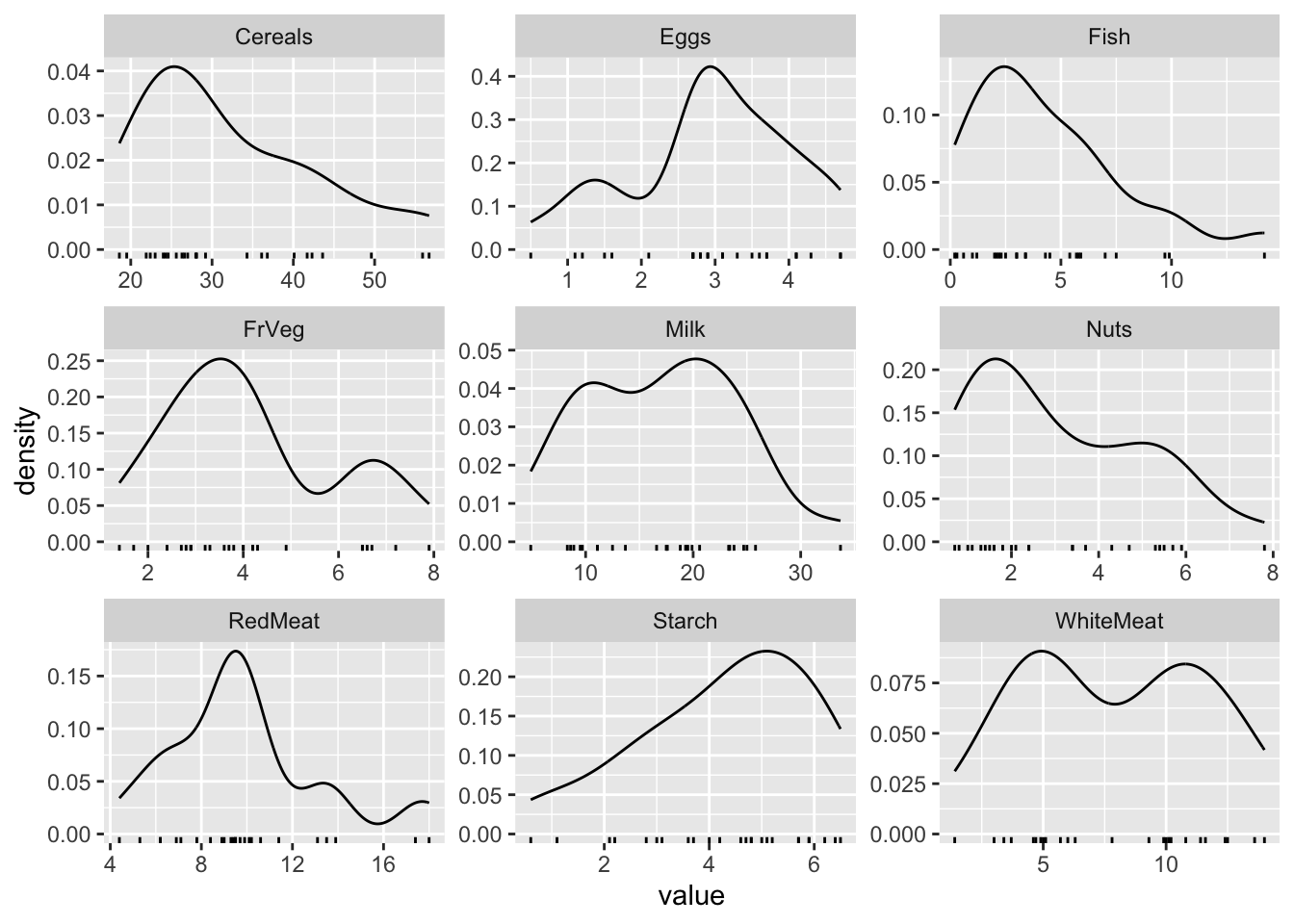
Raw values
tidyr::pivot_longer(d, -Country) %>%
  ggplot(aes(x = name, y = Country, fill = value)) +
  geom_tile() +
  scale_fill_viridis_b()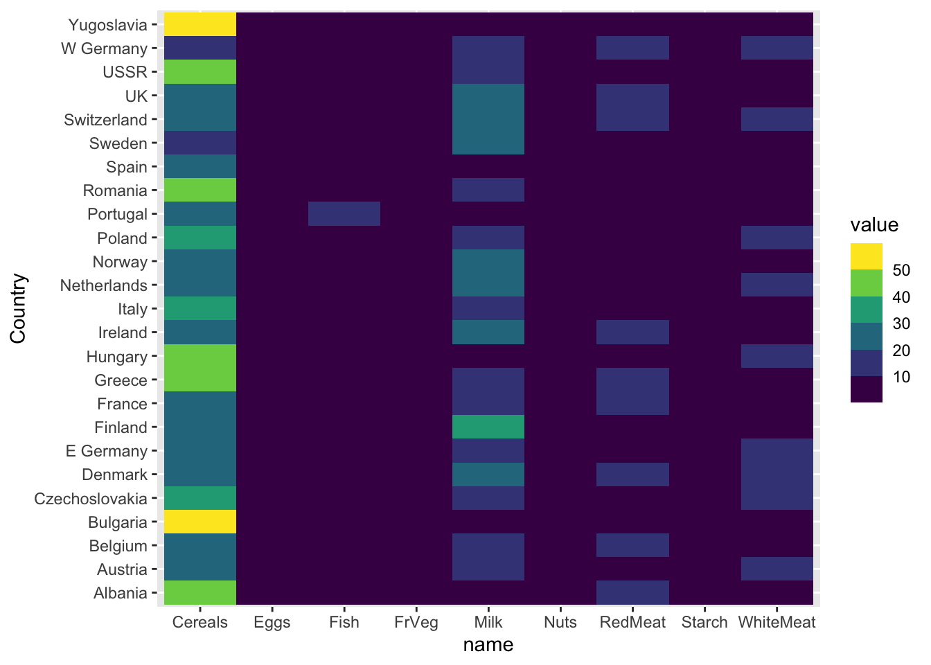
Step 3: Correlations
# scatterplot matrix
car::scatterplotMatrix(d %>% select(-Country), smooth = FALSE)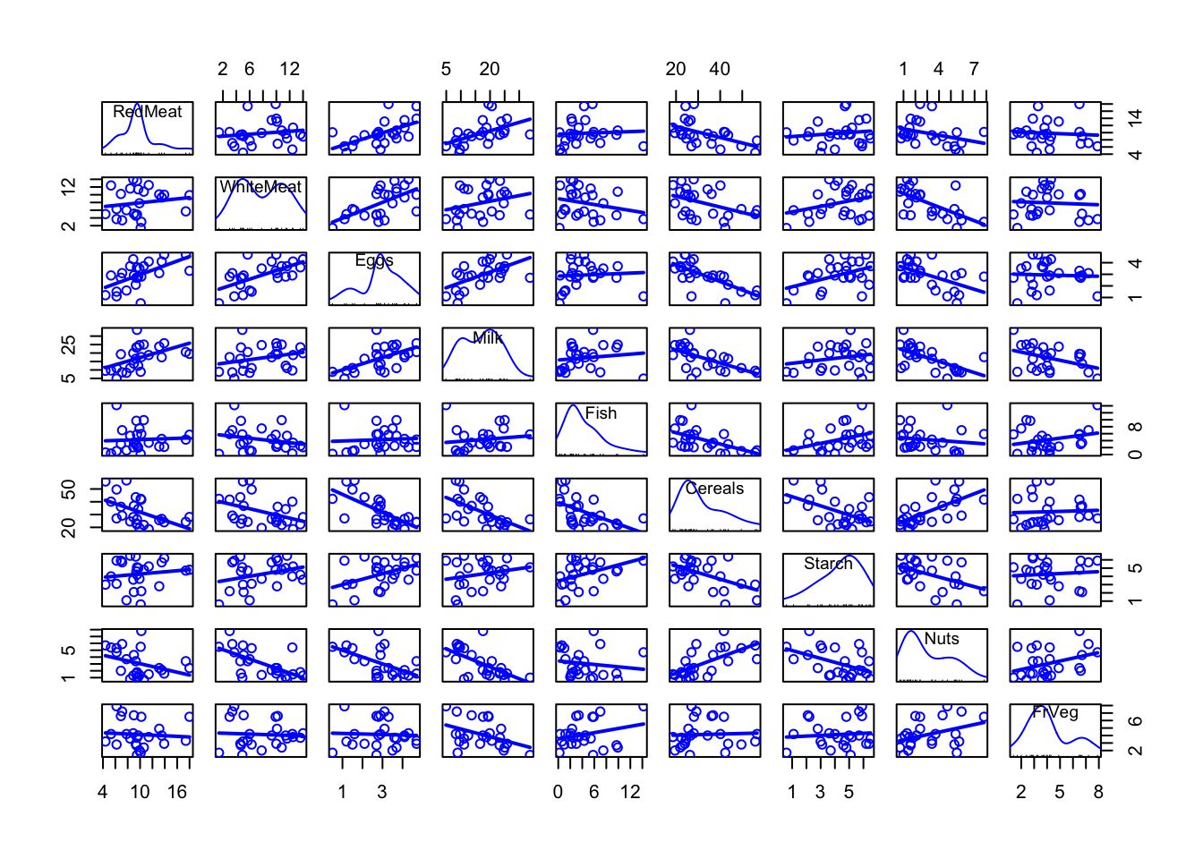
# pairwise correlations
cor(d %>% select(-Country), use = "pairwise.complete.obs")
RedMeat WhiteMeat Eggs Milk Fish Cereals
RedMeat 1.00000000 0.1530027 0.58560895 0.5029311 0.06095745 -0.49987746
WhiteMeat 0.15300271 1.0000000 0.62040916 0.2814839 -0.23400923 -0.41379691
Eggs 0.58560895 0.6204092 1.00000000 0.5755331 0.06557136 -0.71243682
Milk 0.50293110 0.2814839 0.57553312 1.0000000 0.13788370 -0.59273662
Fish 0.06095745 -0.2340092 0.06557136 0.1378837 1.00000000 -0.52423080
Cereals -0.49987746 -0.4137969 -0.71243682 -0.5927366 -0.52423080 1.00000000
Starch 0.13542594 0.3137721 0.45223071 0.2224112 0.40385286 -0.53326231
Nuts -0.34944855 -0.6349618 -0.55978097 -0.6210875 -0.14715294 0.65099727
FrVeg -0.07422123 -0.0613167 -0.04551755 -0.4083641 0.26613865 0.04654808
Starch Nuts FrVeg
RedMeat 0.13542594 -0.3494486 -0.07422123
WhiteMeat 0.31377205 -0.6349618 -0.06131670
Eggs 0.45223071 -0.5597810 -0.04551755
Milk 0.22241118 -0.6210875 -0.40836414
Fish 0.40385286 -0.1471529 0.26613865
Cereals -0.53326231 0.6509973 0.04654808
Starch 1.00000000 -0.4743116 0.08440956
Nuts -0.47431155 1.0000000 0.37496971
FrVeg 0.08440956 0.3749697 1.00000000# same result as a tidy data frame
r <- corrr::correlate(d %>% select(-Country))Correlation computed with
• Method: 'pearson'
• Missing treated using: 'pairwise.complete.obs'corrr::fashion(r, decimals = 1) term RedMeat WhiteMeat Eggs Milk Fish Cereals Starch Nuts FrVeg
1 RedMeat .2 .6 .5 .1 -.5 .1 -.3 -.1
2 WhiteMeat .2 .6 .3 -.2 -.4 .3 -.6 -.1
3 Eggs .6 .6 .6 .1 -.7 .5 -.6 -.0
4 Milk .5 .3 .6 .1 -.6 .2 -.6 -.4
5 Fish .1 -.2 .1 .1 -.5 .4 -.1 .3
6 Cereals -.5 -.4 -.7 -.6 -.5 -.5 .7 .0
7 Starch .1 .3 .5 .2 .4 -.5 -.5 .1
8 Nuts -.3 -.6 -.6 -.6 -.1 .7 -.5 .4
9 FrVeg -.1 -.1 -.0 -.4 .3 .0 .1 .4 # strong correlations to red meat
r %>%
filter(abs(RedMeat) > .5) %>%
select(term, RedMeat)# A tibble: 2 × 2
term RedMeat
<chr> <dbl>
1 Eggs 0.586
2 Milk 0.503# rearrange correlation matrix (uses PCA in the background)
corrr::rearrange(r, absolute = FALSE) %>%
corrr::shave()# A tibble: 9 × 10
term Eggs Milk WhiteMeat RedMeat Starch Fish FrVeg Nuts Cereals
<chr> <dbl> <dbl> <dbl> <dbl> <dbl> <dbl> <dbl> <dbl> <dbl>
1 Eggs NA NA NA NA NA NA NA NA NA
2 Milk 0.576 NA NA NA NA NA NA NA NA
3 WhiteM… 0.620 0.281 NA NA NA NA NA NA NA
4 RedMeat 0.586 0.503 0.153 NA NA NA NA NA NA
5 Starch 0.452 0.222 0.314 0.135 NA NA NA NA NA
6 Fish 0.0656 0.138 -0.234 0.0610 0.404 NA NA NA NA
7 FrVeg -0.0455 -0.408 -0.0613 -0.0742 0.0844 0.266 NA NA NA
8 Nuts -0.560 -0.621 -0.635 -0.349 -0.474 -0.147 0.375 NA NA
9 Cereals -0.712 -0.593 -0.414 -0.500 -0.533 -0.524 0.0465 0.651 NA# heatmap
d %>%
select(-Country) %>%
cor() %>%
ggcorrplot::ggcorrplot() +
scale_fill_viridis_b()Scale for fill is already present.
Adding another scale for fill, which will replace the existing scale.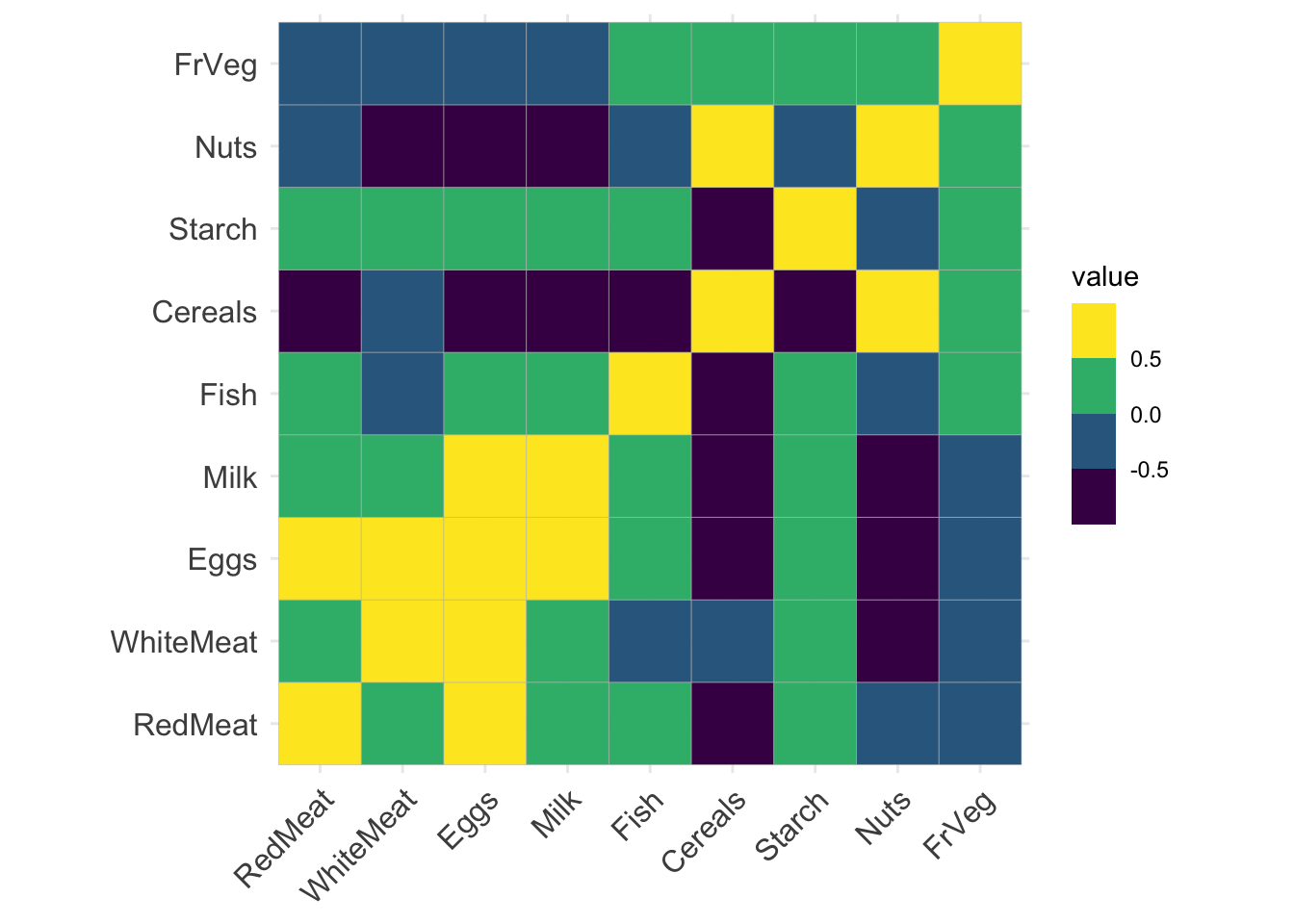
# correlation network
corrr::network_plot(r, curved = FALSE)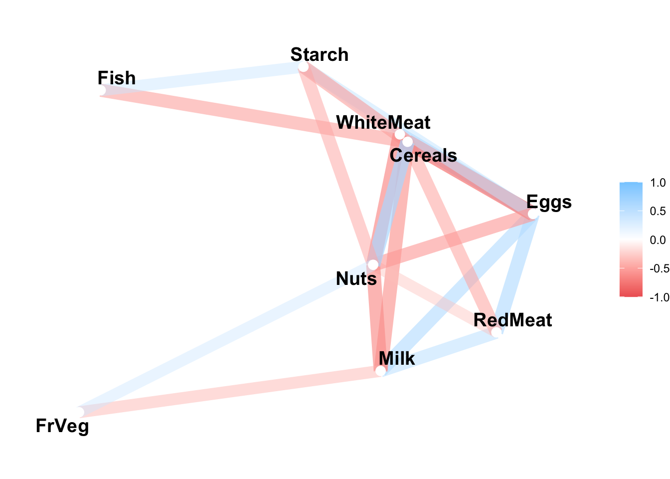
Step 4: Hierarchical Clustering
# rescale the features
rescaled_d <- d %>%
  select(-Country) %>%
  scale()

# add country names on rows
rownames(rescaled_d) <- d$Country
rescaled_d
RedMeat WhiteMeat Eggs Milk Fish
Albania 0.08126490 -1.75848885 -2.17963852 -1.15573814 -1.200282130
Austria -0.27725673 1.65237315 1.22045441 0.39237676 -0.641874675
Belgium 1.09707621 0.38006748 1.04150215 0.05460623 0.063482111
Bulgaria -0.60590157 -0.51325352 -1.19540109 -1.24018077 -0.906383469
Czechoslovakia -0.03824231 0.94854448 -0.12168754 -0.64908235 -0.671264541
Denmark 0.23064892 0.78612248 0.68359763 1.11013912 1.650534878
E Germany -0.42664075 1.00268515 0.68359763 -0.84611516 0.327990905
Finland -0.09799591 -0.81102719 -0.21116367 2.33455726 0.445550369
France 2.44153235 0.54248948 0.32569311 0.33608167 0.416160503
Greece 0.11114171 -1.32536352 -0.12168754 0.06868001 0.474940235
Hungary -1.35282164 1.21924781 -0.03221141 -1.04314796 -1.170892264
Ireland 1.21658342 0.56955981 1.57835893 1.22272929 -0.612484809
Italy -0.24737993 -0.75688652 -0.03221141 -0.48019709 -0.259806416
Netherlands -0.09799591 1.54409181 0.59412150 0.88495877 -0.524315210
Norway -0.12787272 -0.86516785 -0.21116367 0.87088500 1.591755146
Poland -0.87479279 0.62370048 -0.21116367 0.30793413 -0.377365880
Portugal -1.08393041 -1.13587119 -1.64278174 -1.71868901 2.914299118
Romania -1.08393041 -0.43204252 -1.28487722 -0.84611516 -0.965163201
Spain -0.81503919 -1.21708219 0.14674085 -1.19795945 0.798228762
Sweden 0.02151130 -0.02598752 0.50464537 1.06791780 0.945178092
Switzerland 0.97756900 0.59663015 0.14674085 0.94125386 -0.583094943
UK 2.26227153 -0.59446452 1.57835893 0.49089316 0.004702379
USSR -0.15774952 -0.89223819 -0.74802044 -0.07205771 -0.377365880
W Germany 0.46966334 1.24631815 1.04150215 0.23756527 -0.259806416
Yugoslavia -1.62171287 -0.78395685 -1.55330561 -1.07129551 -1.082722666
Cereals Starch Nuts FrVeg
Albania 0.9159176 -2.24957717 1.2227536 -1.35040507
Austria -0.3870690 -0.41368721 -0.8923886 0.09091397
Belgium -0.5146342 0.87143577 -0.4895043 -0.07539207
Bulgaria 2.2280161 -1.94359551 0.3162641 0.03547862
Czechoslovakia 0.1869740 0.44306145 -0.9931096 -0.07539207
Denmark -0.9428885 0.32066878 -1.1945517 -0.96235764
E Germany -0.6968701 1.36100643 -1.1441912 -0.29713346
Finland -0.5419696 0.50425778 -1.0434702 -1.51671112
France -0.3779572 0.32066878 -0.3384228 1.31049162
Greece 0.8612468 -1.27043586 2.3810458 1.31049162
Hungary 0.7154581 -0.16890188 1.1723931 0.03547862
Ireland -0.7515408 1.17741743 -0.7413070 -0.68518090
Italy 0.4147689 -1.33163219 0.6184273 1.42136232
Netherlands -0.8973295 -0.04650921 -0.6405859 -0.24169812
Norway -0.8426588 0.19827612 -0.7413070 -0.79605159
Poland 0.3509863 0.99382843 -0.5398649 1.36592697
Portugal -0.4781870 0.99382843 0.8198694 2.08658649
Romania 1.5810786 -0.71966887 1.1220326 -0.74061625
Spain -0.2777275 0.87143577 1.4241958 1.69853906
Sweden -1.1615716 -0.35249087 -0.8420280 -1.18409903
Switzerland -0.6057521 -0.90325786 -0.3384228 0.42352606
UK -0.7242054 0.25947245 0.1651825 -0.46343951
USSR 1.0343709 1.29981010 0.1651825 -0.68518090
W Germany -1.2435778 0.56545411 -0.7916675 -0.18626277
Yugoslavia 2.1551217 -0.78086520 1.3234747 -0.51887486
attr(,"scaled:center")
RedMeat WhiteMeat Eggs Milk Fish Cereals Starch Nuts
9.828 7.896 2.936 17.112 4.284 32.248 4.276 3.072
FrVeg
4.136
attr(,"scaled:scale")
RedMeat WhiteMeat Eggs Milk Fish Cereals Starch Nuts
3.347078 3.694081 1.117617 7.105416 3.402533 10.974786 1.634085 1.985682
FrVeg
1.803903 # get Euclidean distances
distance_m <- dist(rescaled_d, method = "euclidean")
distance_m Albania Austria Belgium Bulgaria Czechoslovakia Denmark
Austria 6.1360510
Belgium 5.9487614 2.4513223
Bulgaria 2.7645367 4.9002772 5.2370880
Czechoslovakia 5.1411480 2.1308906 2.2202549 3.9503627
Denmark 6.6341625 3.0192376 2.5391149 6.0365915 3.3692190
E Germany 6.3922502 2.5819811 2.1140954 5.4091332 1.8802660 2.7645740
Finland 5.8794649 4.0716662 3.5042937 5.8176296 3.9839792 2.6334871
France 6.3070106 3.5889373 2.1944157 5.5606801 3.3690903 3.6628201
Greece 4.2559301 5.1639348 4.6951531 3.7626971 4.8701393 5.5968794
Hungary 4.6734470 3.2857392 3.9946781 3.3453809 2.7513287 5.0390826
Ireland 6.7571210 2.7408193 1.6567570 6.2125897 3.1576644 2.8295563
Italy 4.0255665 3.7175506 3.7186963 2.8654638 3.3461638 4.7794027
Netherlands 6.0080723 1.1233122 2.2489670 5.1685911 2.1938164 2.5365988
Norway 5.4652307 3.8755033 2.9606943 5.2768296 3.5270340 1.9936668
Poland 5.8828058 2.7959971 2.9359042 4.4345191 2.1044427 3.8446943
Portugal 6.6120099 6.5291699 5.6512736 6.0046278 5.5189793 5.8699772
Romania 2.6895968 4.6504990 4.7603534 1.8894354 3.5622341 5.5339127
Spain 5.5683482 4.8880906 3.9977053 4.8419395 4.1491845 5.1119708
Sweden 5.6536745 2.9369074 2.5853728 5.3969214 3.2573130 1.3816672
Switzerland 5.1237136 2.2026742 2.3442632 4.4827981 2.6235926 3.1882479
UK 5.9403845 3.7477881 1.9460278 5.7960604 3.8309331 3.4750112
USSR 4.3453152 4.1625991 3.1606186 3.8308791 2.7166105 4.1618777
W Germany 6.3546987 1.6443946 1.4179580 5.6109214 2.1838999 2.3922302
Yugoslavia 2.9423491 5.4454697 5.6037933 1.9929633 4.3406075 6.3622057
E Germany Finland France Greece Hungary Ireland
Austria
Belgium
Bulgaria
Czechoslovakia
Denmark
E Germany
Finland 4.0723681
France 3.7933343 4.5951025
Greece 5.6196014 5.5036614 4.5450471
Hungary 3.6762821 5.3948141 4.9747050 4.1100241
Ireland 3.0335760 3.2360376 3.1517086 5.7045668 4.8176916
Italy 4.3204290 4.9150443 3.8021484 2.1501238 3.1534119 4.8438555
Netherlands 2.5318280 3.3844709 3.4081356 5.1560504 3.4911095 2.3440329
Norway 3.2723624 2.0626772 3.9205053 4.6276066 4.9080845 3.6097337
Poland 2.7089165 4.1287431 3.5988128 4.4141412 3.0425352 3.7374057
Portugal 5.2526342 6.5077018 5.6560241 4.7836767 5.6978958 7.0636496
Romania 4.7841740 5.0667941 5.5261450 3.6198948 2.4712108 5.6047613
Spain 4.0873016 5.4810616 4.4501043 3.0986288 3.8802367 5.2828595
Sweden 3.0603112 2.0654515 3.8171890 4.9853695 4.6652093 2.8554901
Switzerland 3.5712007 3.5373183 2.4247646 4.1069156 3.8538000 2.8159357
UK 3.9281144 3.8829048 2.5712483 4.6219345 5.1192989 2.2537043
USSR 3.4169052 3.4694963 4.2371627 4.1142825 3.4299121 3.8981565
W Germany 1.8918353 3.6535570 2.9355723 5.3638262 3.9024547 1.8075098
Yugoslavia 5.5249305 5.7951005 6.3060106 3.9306646 3.0306252 6.4616924
Italy Netherlands Norway Poland Portugal Romania
Austria
Belgium
Bulgaria
Czechoslovakia
Denmark
E Germany
Finland
France
Greece
Hungary
Ireland
Italy
Netherlands 3.9200450
Norway 3.9999099 3.3633647
Poland 3.1182065 2.7728627 3.7069384
Portugal 4.6620200 6.3696842 4.7962996 4.8153273
Romania 3.1094185 4.6422159 4.6832317 3.9543844 5.6299298
Spain 2.8739888 4.8662539 4.1615640 3.3982806 2.9327729 4.2425253
Sweden 4.1362186 2.4025962 1.5038553 3.8417285 5.8691378 4.8593580
Switzerland 2.9369672 1.9010940 3.3378230 3.0735117 6.1223699 4.3591550
UK 4.1855029 3.5171274 3.5498903 4.4995477 6.5379656 5.4235820
USSR 3.5595624 3.8817620 3.2599160 2.9171227 5.0751340 2.7565008
W Germany 4.1372575 1.2729590 3.2990760 2.9969977 6.1423089 5.0906052
Yugoslavia 3.5810088 5.5029824 5.4083224 4.4910456 5.8259987 0.9862315
Spain Sweden Switzerland UK USSR W Germany
Austria
Belgium
Bulgaria
Czechoslovakia
Denmark
E Germany
Finland
France
Greece
Hungary
Ireland
Italy
Netherlands
Norway
Poland
Portugal
Romania
Spain
Sweden 4.8090500
Switzerland 4.5800551 2.6892031
UK 4.7140258 3.1327459 2.8413601
USSR 3.6276949 3.7704135 3.7949652 4.0055168
W Germany 4.6031064 2.4691803 2.2850740 2.8948301 3.8951198
Yugoslavia 4.5671022 5.7021369 5.2095925 6.2665008 3.3546971 5.9638408# hierarchical clustering
clusters_d <- hclust(distance_m, method = "ward.D")
clusters_d
Call:
hclust(d = distance_m, method = "ward.D")

Cluster method   : ward.D
Distance         : euclidean
Number of objects: 25 str(clusters_d)List of 7
$ merge : int [1:24, 1:2] -18 -2 -6 -3 -12 -15 -5 -10 -4 -21 ...
$ height : num [1:24] 0.986 1.123 1.382 1.418 1.837 ...
$ order : int [1:25] 8 15 6 20 11 23 16 5 7 21 ...
$ labels : chr [1:25] "Albania" "Austria" "Belgium" "Bulgaria" ...
$ method : chr "ward.D"
$ call : language hclust(d = distance_m, method = "ward.D")
$ dist.method: chr "euclidean"
- attr(*, "class")= chr "hclust"# dendrogram with k = 2 clusters
factoextra::fviz_dend(clusters_d, k = 2, rect = TRUE)Warning: The `<scale>` argument of `guides()` cannot be `FALSE`. Use "none" instead as
of ggplot2 3.3.4.
ℹ The deprecated feature was likely used in the factoextra package.
Please report the issue at <https://github.com/kassambara/factoextra/issues>.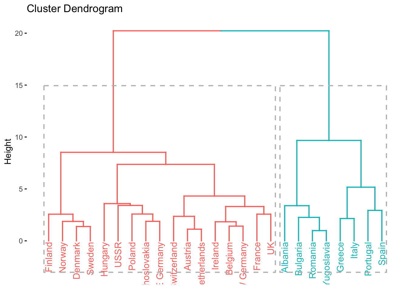
# dendrogram with k = 3 clusters
factoextra::fviz_dend(clusters_d, k = 3, rect = TRUE)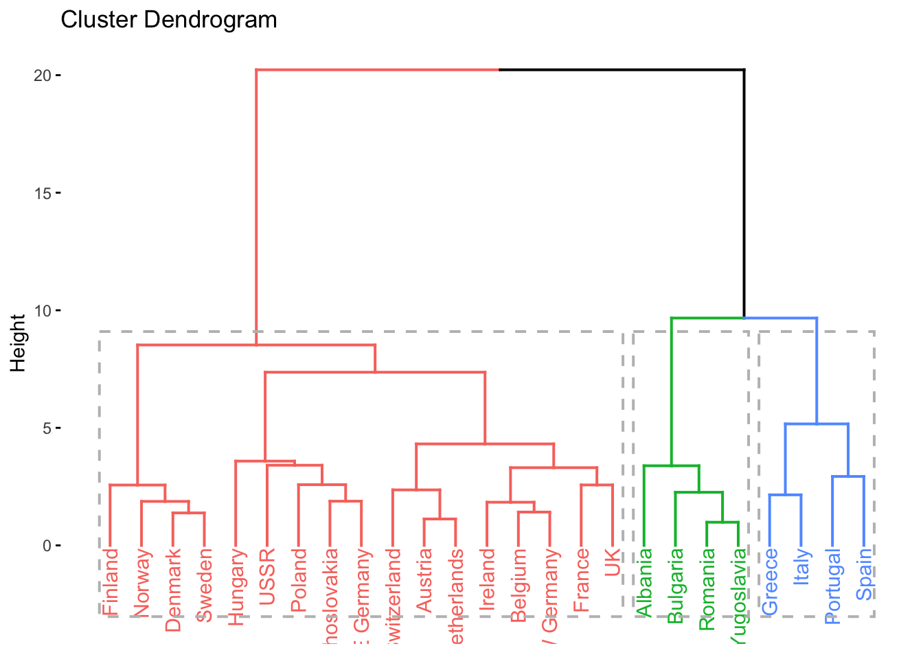
# dendrogram with k = 4 clusters
factoextra::fviz_dend(clusters_d, k = 4, rect = TRUE)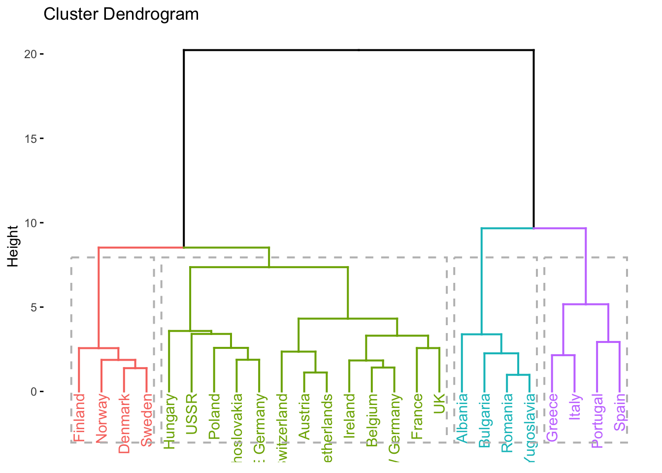
# dendrogram with k = 5 clusters
factoextra::fviz_dend(clusters_d, k = 5, rect = TRUE)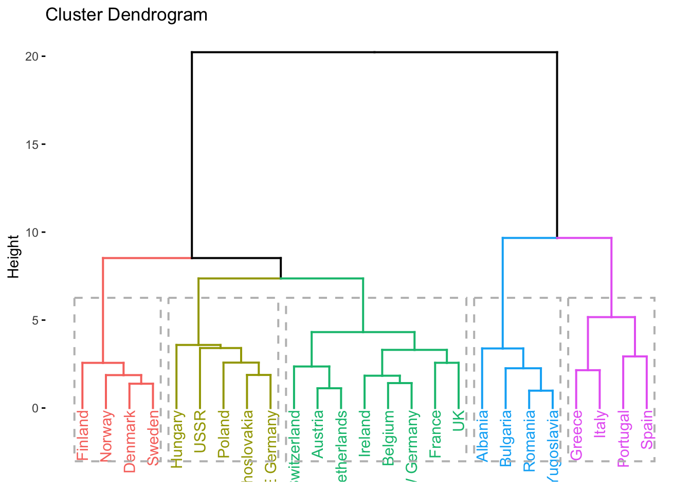
# base R heatmap for dendrograms on both sides
heatmap(rescaled_d)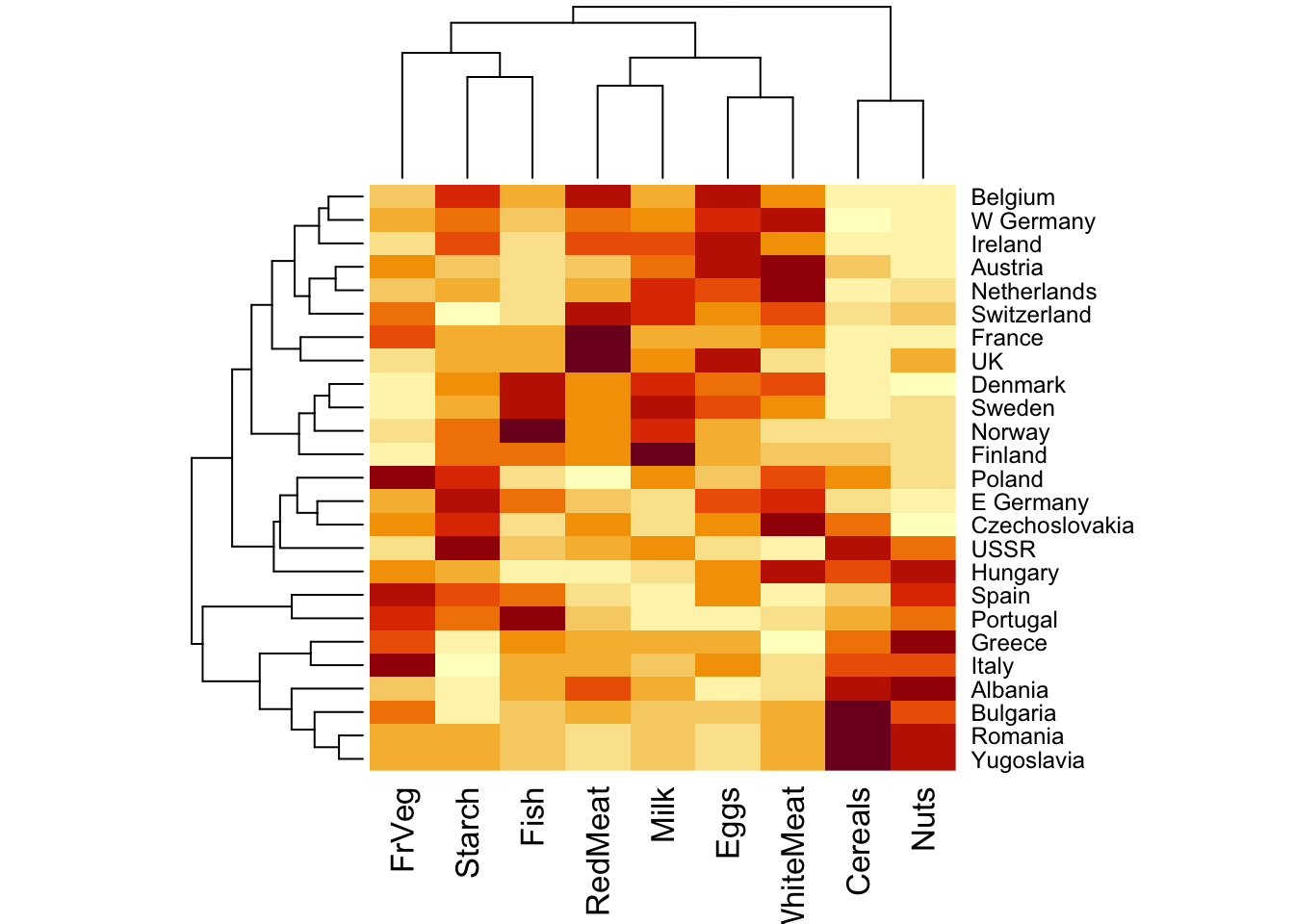
Step 5: K-Means
plotly is an R interface to the Plotly JavaScript visualization library, which has its own features and syntax: https://plotly.com/r/.
# use the rescaled data
k <- kmeans(rescaled_d, centers = 3, iter.max = 10)
str(k)
List of 9
$ cluster : Named int [1:25] 1 2 2 1 2 2 2 2 2 1 ...
..- attr(*, "names")= chr [1:25] "Albania" "Austria" "Belgium" "Bulgaria" ...
$ centers : num [1:3, 1:9] -0.61 0.452 -0.949 -0.655 0.506 ...
..- attr(*, "dimnames")=List of 2
.. ..$ : chr [1:3] "1" "2" "3"
.. ..$ : chr [1:9] "RedMeat" "WhiteMeat" "Eggs" "Milk" ...
$ totss : num 216
$ withinss : num [1:3] 39.2 63 4.3
$ tot.withinss: num 106
$ betweenss : num 110
$ size : int [1:3] 8 15 2
$ iter : int 2
$ ifault : int 0
- attr(*, "class")= chr "kmeans"# cluster assignments
k$cluster Albania Austria Belgium Bulgaria Czechoslovakia
1 2 2 1 2
Denmark E Germany Finland France Greece
2 2 2 2 1
Hungary Ireland Italy Netherlands Norway
1 2 1 2 2
Poland Portugal Romania Spain Sweden
2 3 1 3 2
Switzerland UK USSR W Germany Yugoslavia
2 2 1 2 1 # distances to each centroid
k$centers RedMeat WhiteMeat Eggs Milk Fish Cereals Starch
1 -0.6096362 -0.6553728 -0.8934192 -0.7300065 -0.6859595 1.2382474 -0.8956083
2 0.4517373 0.5063957 0.5762263 0.5837801 0.1183432 -0.6100043 0.3533068
3 -0.9494848 -1.1764767 -0.7480204 -1.4583242 1.8562639 -0.3779572 0.9326321
Nuts FrVeg
1 1.0401967 -0.06153324
2 -0.7043759 -0.21952398
3 1.1220326 1.89256278# sum-of-squares of each cluster
k$withinss[1] 39.167085 62.969328 4.300578# plot clusters (using PCA for axes)
autoplot(k, data = rescaled_d, frame = TRUE, frame.type = "t", label = TRUE)Too few points to calculate an ellipse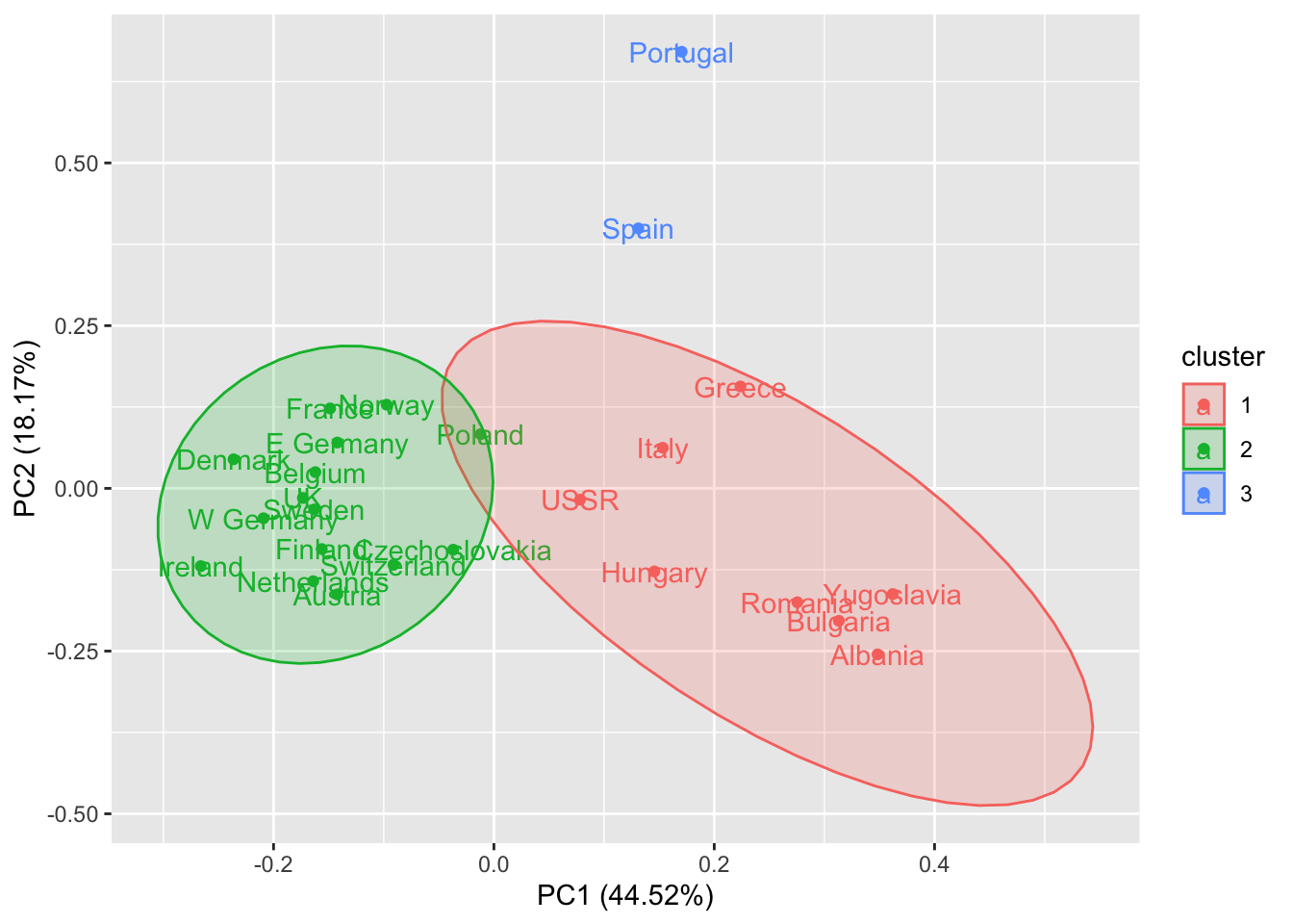
# [NOTE] the function above works through two packages: {ggplot2} provides the
# `autoplot` function, which looks for a plotting method suitable for objects
# of class `kmeans`, because that's the class of the `k` object; the plotting
# method itself is provided by the {ggfortify} package.

# experiment with fewer/more clusters
autoplot(kmeans(rescaled_d, 2), data = rescaled_d, frame = TRUE, label = TRUE)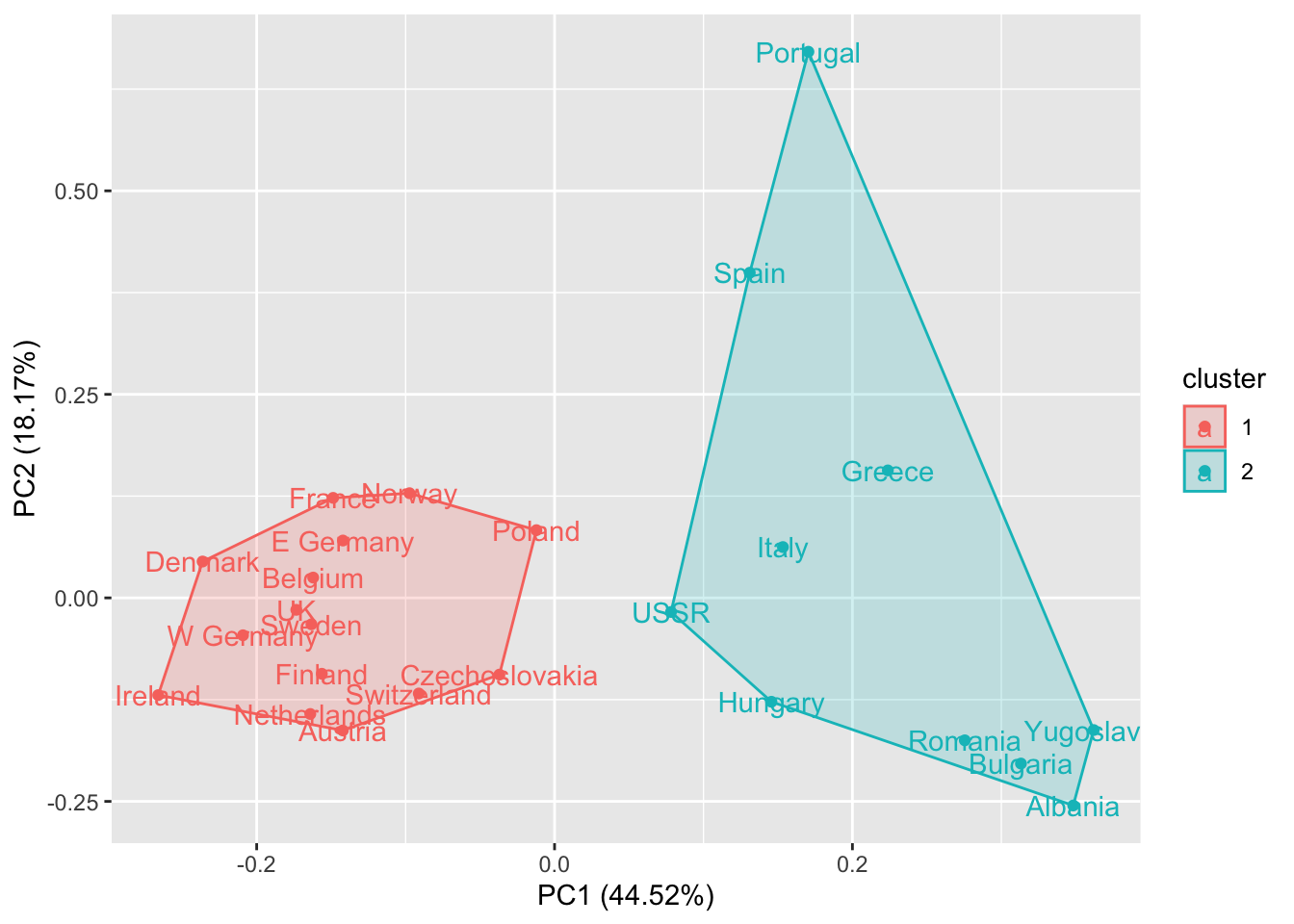
autoplot(kmeans(rescaled_d, 4), data = rescaled_d, frame = TRUE, label = TRUE)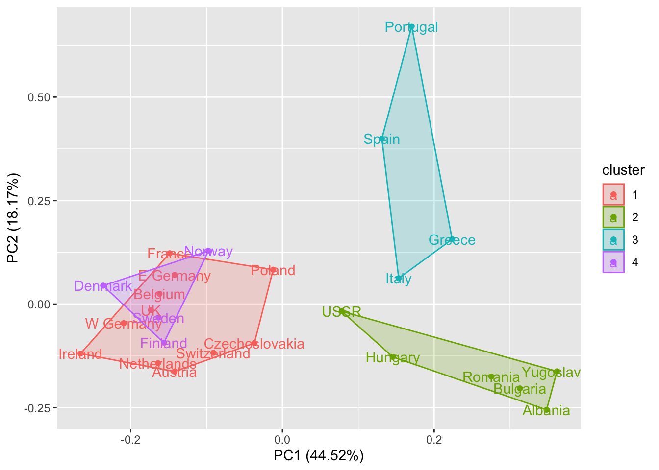
# combine clusters to rescaled data
k <- bind_cols(rescaled_d, Country = d$Country, cluster = factor(k$cluster))

# 2-dimensional view, using red meat and cereals
ggplot(k, aes(x = RedMeat, y = Cereals, color = cluster)) +
  geom_text(aes(label = Country))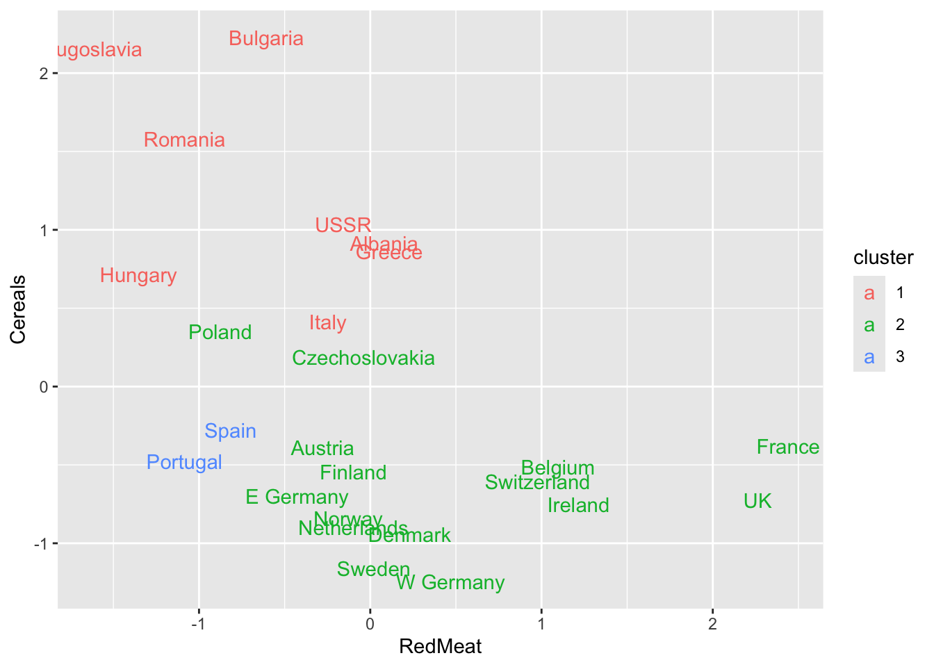
# 3-dimensional view, adding milk
plotly::plot_ly(
  data = k,
  x = ~ RedMeat,
  y = ~ Cereals,
  z = ~ Milk,
  color = ~ cluster,
  type = "scatter3d",
  mode = "markers"
)
Source
Data source: Weber, A. (1973) Agrarpolitik im Spannungsfeld der internationalen Ernaehrungspolitik, Institut fuer Agrarpolitik und marktlehre, Kiel.
The data were fetched from the GitHub repository for Nina Zumel and John Mount, Practical Data Science with R, 2nd edition, Manning 2019. Please refer to that source for additional details on the data.