Exercise 2: Feelings towards French politicians, 2017

Session 12

Most PCA code from Waggoner 2021, ch. 2

Download datasets on your computer

1. CN4France2017.Fin.sav.

Step 1: Load data and install useful packages

library(tidyverse) # {dplyr}, {ggplot2}, {readxl}, {stringr}, {tidyr}, etc.

library(corrr)
library(factoextra)

Welcome! Want to learn more? See two factoextra-related books at https://goo.gl/ve3WBa

library(ggrepel)

repository <- "data"

#CNEP French survey
d <- haven::read_sav(paste0(repository, "/CN4France2017.Fin.sav"))

Step 2: Explore

table(d$Q14)

  1   2   3   4   5   6   7   8   9  10 
 60 110 229 170 646 197 180 179  84 143 

table(d$Q19a_a)

  0   1   2   3   4   5   6   7   8   9  10 
533 183 225 196 158 360 122 105  63  24  27 

# select 'thermometer' (feelings towards...) variables
p <- select(d, starts_with("Q19"))

# average feeling scores
apply(p, 2, mean, na.rm = TRUE)

  Q19a_a   Q19a_b   Q19a_c   Q19a_d   Q19a_e   Q19a_f   Q19a_g   Q19a_h 
3.061122 4.752876 3.754386 2.696894 3.126881 4.661993 4.111222 2.129760 
  Q19a_i   Q19a_j   Q19a_k   Q19a_l   Q19a_m 
2.548823 2.988448 3.696241 3.020551 3.384577 

# rename columns
names(p) <- sapply(names(p), function(x) attr(p[[x]], "label"))
names(p) <- stringr::str_remove(names(p), ".*group - ")
# View(p)

Step 3: Correlation

# heatmap
cor(p, use = "pairwise.complete.obs") %>%
  ggcorrplot::ggcorrplot() +
  scale_fill_viridis_b()

Scale for fill is already present.
Adding another scale for fill, which will replace the existing scale.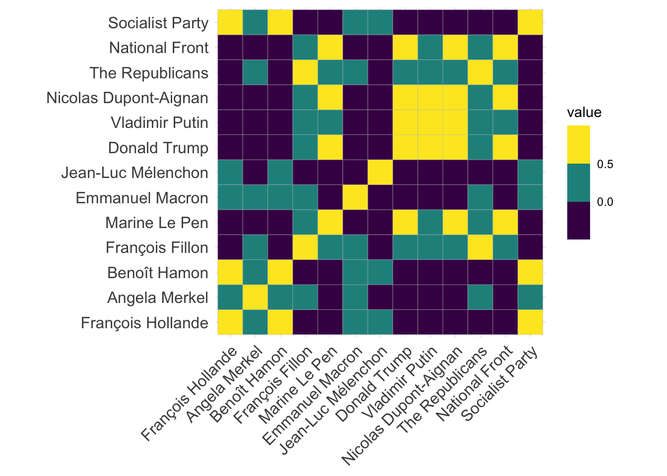

# network
cor(p, use = "pairwise.complete.obs") %>%
  corrr::network_plot(curved = FALSE)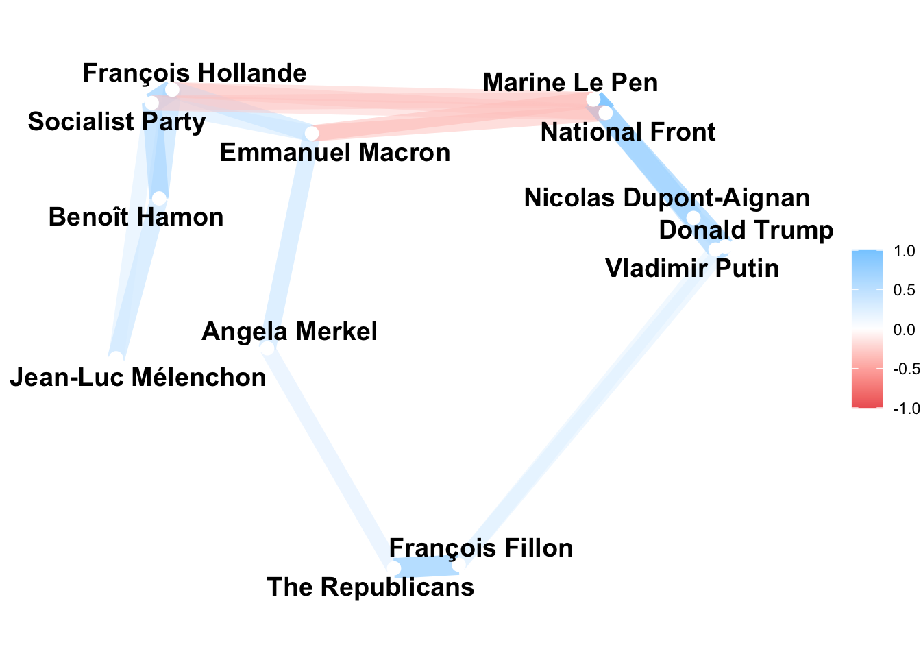

Principal Components

pca_fit <- p %>%
  na.omit() %>%
  scale(center = TRUE, scale = TRUE) %>%
  prcomp()

summary(pca_fit)

Importance of components:
                          PC1    PC2    PC3     PC4    PC5     PC6     PC7
Standard deviation     2.1439 1.5204 1.3879 0.92610 0.8292 0.74860 0.65762
Proportion of Variance 0.3536 0.1778 0.1482 0.06597 0.0529 0.04311 0.03327
Cumulative Proportion  0.3536 0.5314 0.6795 0.74553 0.7984 0.84153 0.87480
                           PC8    PC9    PC10    PC11    PC12    PC13
Standard deviation     0.60631 0.5858 0.56680 0.52172 0.49089 0.28708
Proportion of Variance 0.02828 0.0264 0.02471 0.02094 0.01854 0.00634
Cumulative Proportion  0.90308 0.9295 0.95419 0.97512 0.99366 1.00000

# variance explained per component
variance <- tibble(
  var = pca_fit$sdev^2,
  var_exp = var / sum(var),
  cum_var_exp = cumsum(var_exp)
) %>%
  mutate(pc = row_number())

# proportion of variance explained (PVE)
ggplot(variance, aes(pc, var_exp)) +
  geom_point() +
  geom_line() +
  geom_label_repel(aes(label = pc), size = 4) +
  labs(x = "Principal Component", y = "PVE") +
  scale_y_continuous(labels = scales::percent)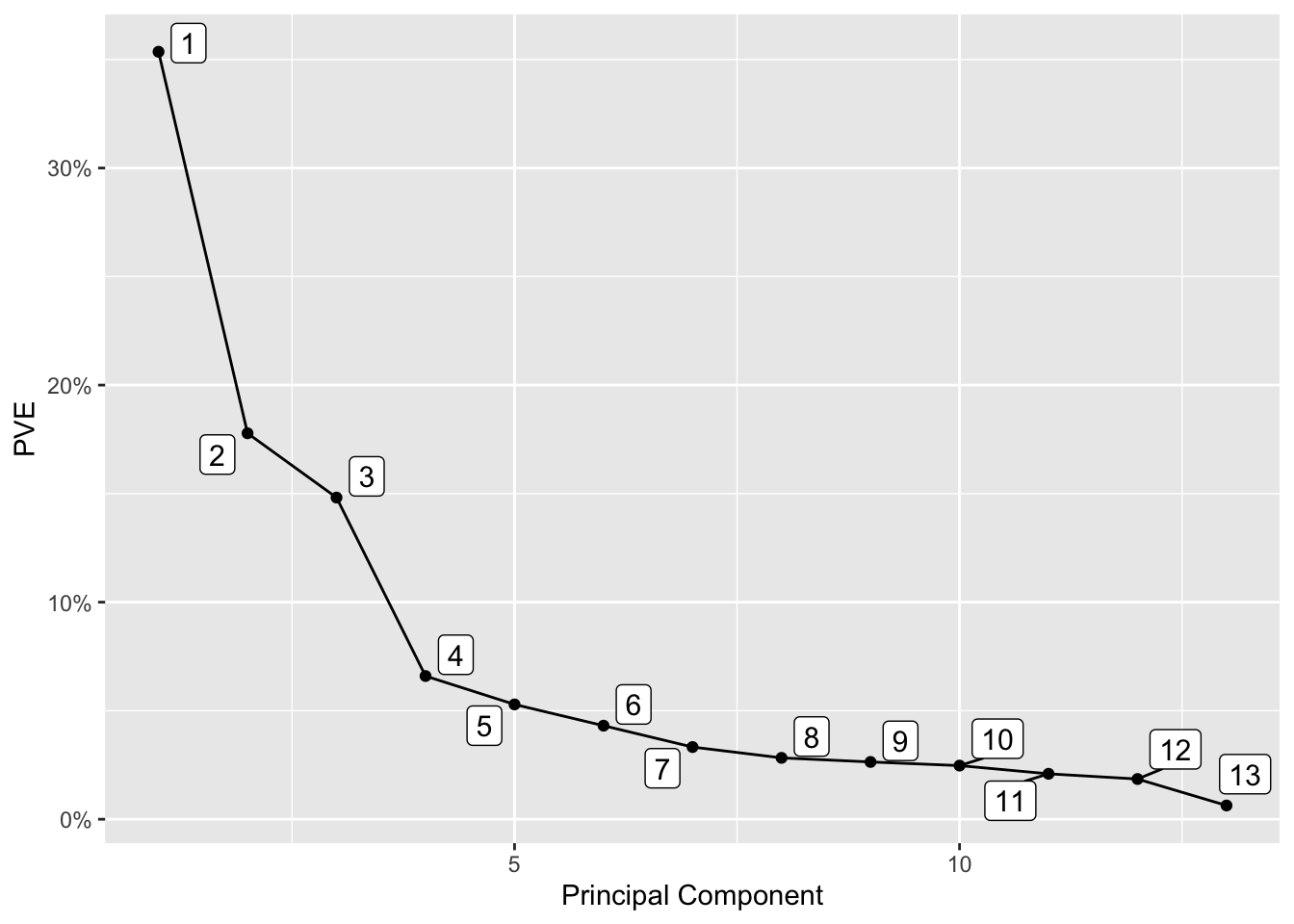

# same plot ('scree plot') using {factoextra}
fviz_screeplot(pca_fit, addlabels = TRUE, choice = "variance")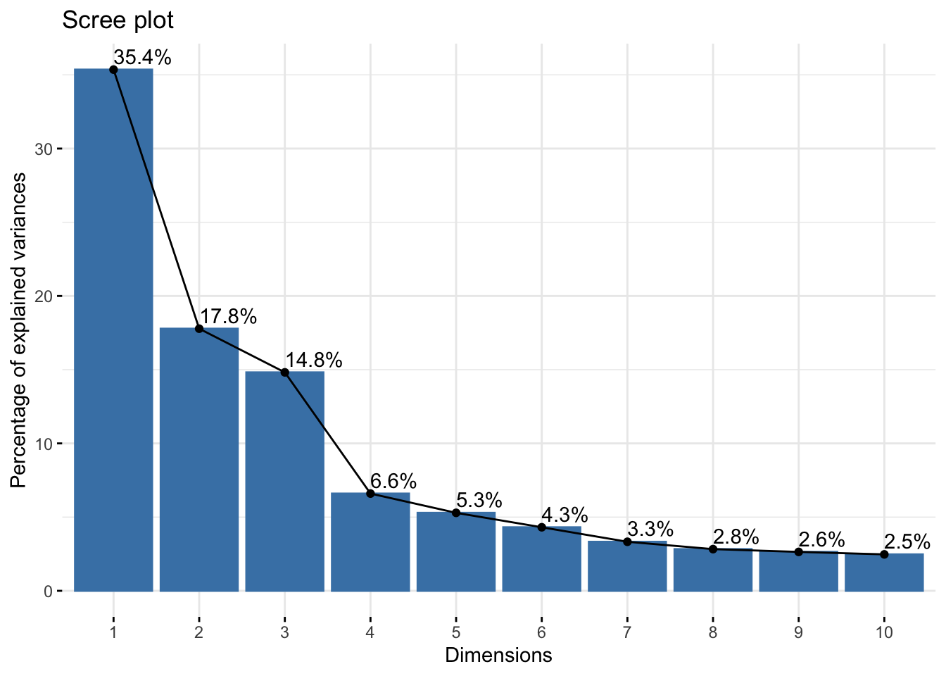

# 'biplot'
fviz_pca_biplot(pca_fit, label = "var", col.var = "black", col.ind = "grey80")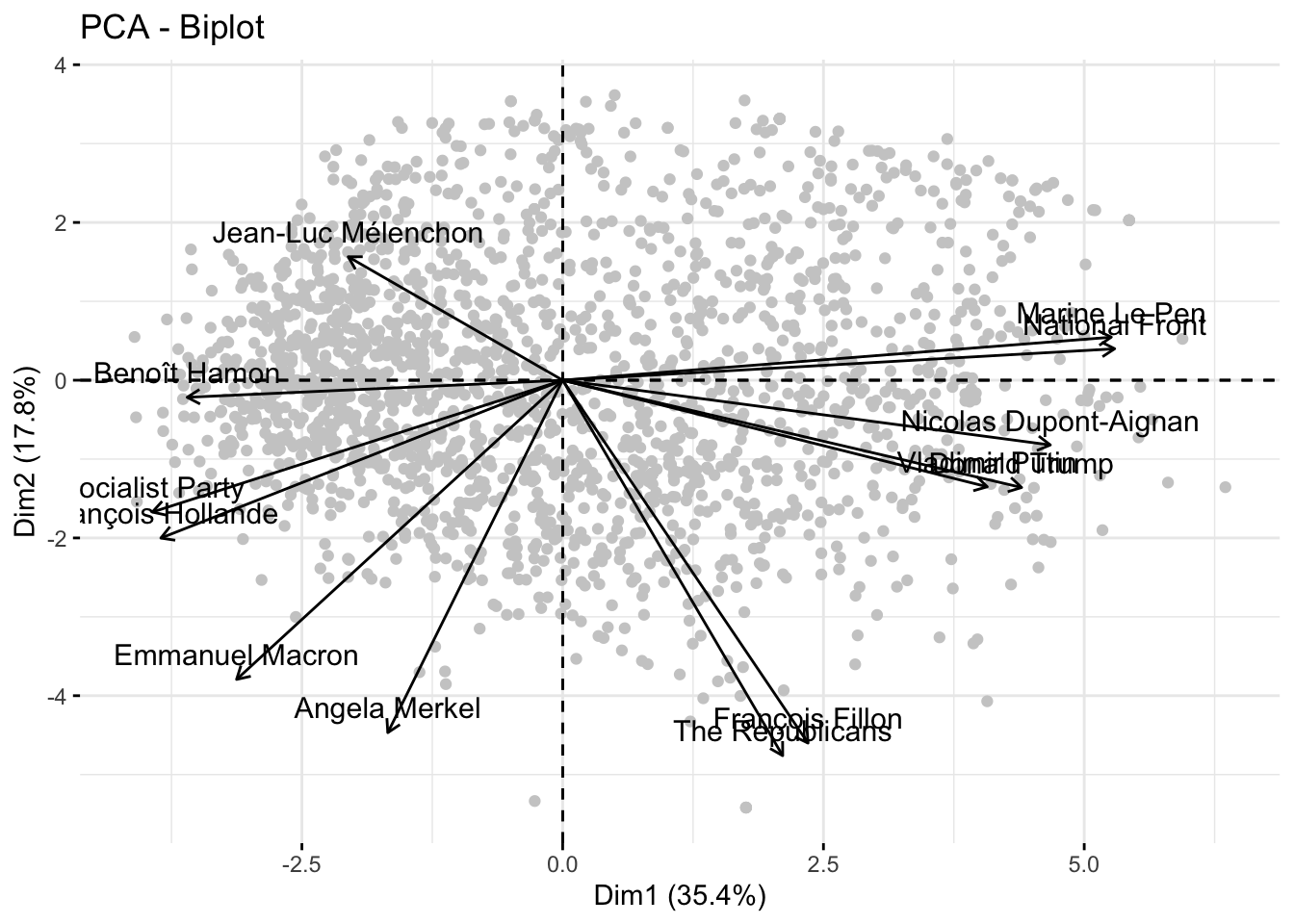

# feature loadings/contributions ("contrib")
pca_fit %>%
  fviz_pca_var(col.var = "contrib") +
  scale_color_gradient(low = "grey50", high = "tomato") +
  labs(color = "Contribution", title = "") +
  theme_minimal()+
  theme(axis.title = element_text(size=15),
        axis.text = element_text(size=17))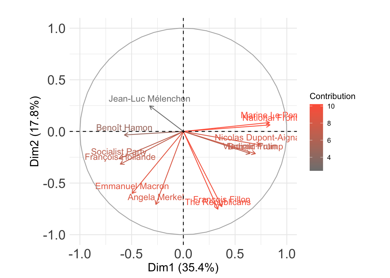

# show relationship to ideology
tibble(
  `PC 1` = pca_fit$x[, 1],
  `PC 2` = pca_fit$x[, 2],
  `Left-Right` = as.integer(d$Q14[ -attr(na.omit(p), "na.action") ])
) %>%
  ggplot(aes(`PC 1`, `PC 2`, color = `Left-Right`)) +
  geom_point() +
  scale_color_viridis_b()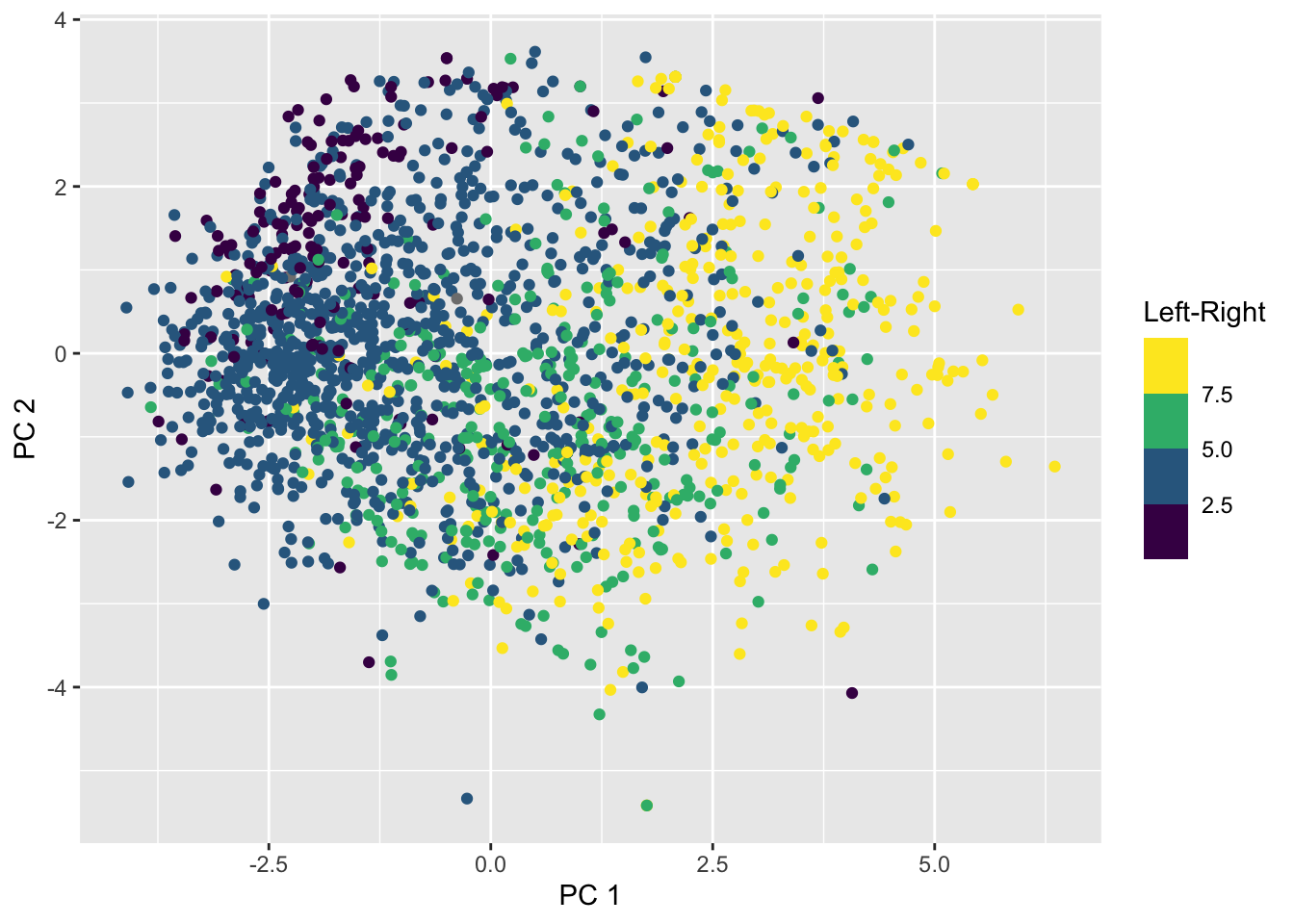

# ... or, in combination to biplot
fviz_pca_biplot(
  pca_fit,
  label = "var",
  col.var = "black",
  col.ind = as.integer(d$Q14[ -attr(na.omit(p), "na.action") ]),
  alpha.ind = 0.5
) +
  scale_color_viridis_b()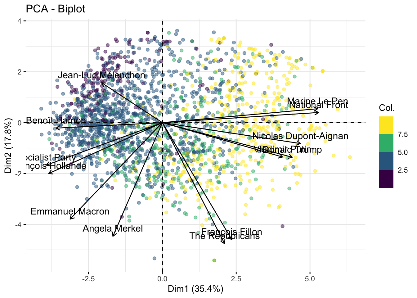

Source

Data source: Comparative National Elections Project (CNEP), 2017 CNEP France Survey, 2017.

More details on the data can be obtained from the CNEP website.

The full data are provided in zipped SPSS format, but please do not redistribute and redirect users to the CNEP website instead.