Linear Regression

Session 9

François Briatte
(small modifs by Kim Antunez & ChatGPT)

2024-04-02

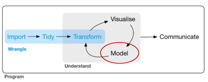
Modeling

One of the key steps of DataScience

1. Choose a Model

Based on the hypothesis, you select a mathematical model or equation that you believe describes the relationship within the data. The choice of the model depends on the nature of the data and the research question. Models can be linear, nonlinear, simple, or complex.

2. Fitting the Model (an equation through the data)

The next step is to estimate the model’s parameters to make it align as closely as possible with the observed data. The process of estimating these parameters is often called “fitting the model” to the data. The goal is to find the best-fitting model that minimizes the difference (usually a measure of error) between the model’s predictions and the actual data points.

3. Formulate interpretable statements

Once the model is fit, it can help you understand the underlying relationships in the data. You can extract coefficients and other information from the model to make interpretable statements or draw conclusions. Tests can help for this step.

What a model does for you?

A model is a fundamental tool in data analysis and statistics that helps researchers and analysts make sense of data by unifying events into a structured process, providing insights, and serving as a descriptive instrument for understanding trends, changes, forecasting, and latent patterns in the data. It’s a valuable means of simplifying complex phenomena, enabling better decision-making, and gaining actionable insights. More precisely:

Unifies observations into a data-Generating process

(structured and organized manner to represent real-world phenomena)

Example: In a linear regression model, events and observations (data points) are unified through a linear equation that represents the relationship between variables

Provides corresponding insight on that process

Thanks to the use of mathematical equations, parameters, and coefficients you can see relationships between variables that might not be apparent when examining raw data.

Serves as an instrument to describe

General Trends in the Data: On average, when sales are higher, advertising spending increase
Marginal Changes to the Data: Controlling for factors like work experience, location, and gender, a multiple linear regression model reveals the isolated impact of education on income.
Future Scenarios (Forecasting): Controlling for various economic factors, a time series model can be employed to forecast future stock prices
Latent Classes in the Data (Clustering, Partitioning): Reveal distinct customer segments, allowing a business to tailor marketing strategies to different customer groups based on their preferences and behavior.

All models are wrong, but some are useful. – [George Box]

This quote highlights that while no model perfectly represents the real world, they can still be valuable tools for describing and understanding complex systems. Models provide a simplification of reality, making it more manageable for analysis and decision-making.

What a LINEAR model does for you?

A linear model is a powerful tool that helps you find the best-fitting linear relationship in your data, provides interpretable parameters, and offers valuable insights into the goodness of fit and residual analysis. These models are robust, user-friendly, and suitable for various analytical tasks. More precisely:

Identifies the Best Linear Fit: parameters (coefficients) that minimize the difference between the observed values and the values predicted by the linear equation (squared error term)
Interpretable Parameters: In a linear regression predicting the price of a house (dependent variable in euro) based on its surface area (independent variable in square meters), a coefficient of 100 for surface area means that for each additional square meter of surface area, the house’s price is expected to increase by 100 euros, assuming all other factors remain the same.
Goodness-of-fit: R-squared tells you how well the model explains the variance in the dependent variable.
Robust and Simple: Linear models don’t require advanced mathematical techniques and perform reasonably well even when some of their underlying assumptions are violated.

Before Exercise 1

Example

The mtcars dataset contains information about various car models.

# Load the mtcars dataset
data(mtcars)

# Preview
head(mtcars)

                   mpg cyl disp  hp drat    wt  qsec vs am gear carb
Mazda RX4         21.0   6  160 110 3.90 2.620 16.46  0  1    4    4
Mazda RX4 Wag     21.0   6  160 110 3.90 2.875 17.02  0  1    4    4
Datsun 710        22.8   4  108  93 3.85 2.320 18.61  1  1    4    1
Hornet 4 Drive    21.4   6  258 110 3.08 3.215 19.44  1  0    3    1
Hornet Sportabout 18.7   8  360 175 3.15 3.440 17.02  0  0    3    2
Valiant           18.1   6  225 105 2.76 3.460 20.22  1  0    3    1

# Fit a simple linear regression model to predict miles per gallon (`mpg`)
# based on the number of cylinders (`cyl`).
lm_model <- lm(mpg ~ cyl, data = mtcars)

# Print the summary of the regression model (estimated coefficients, residuals, R-squared value...).
summary(lm_model)


Call:
lm(formula = mpg ~ cyl, data = mtcars)

Residuals:
    Min      1Q  Median      3Q     Max 
-4.9814 -2.1185  0.2217  1.0717  7.5186 

Coefficients:
            Estimate Std. Error t value Pr(>|t|)    
(Intercept)  37.8846     2.0738   18.27  < 2e-16 ***
cyl          -2.8758     0.3224   -8.92 6.11e-10 ***
---
Signif. codes:  0 '***' 0.001 '**' 0.01 '*' 0.05 '.' 0.1 ' ' 1

Residual standard error: 3.206 on 30 degrees of freedom
Multiple R-squared:  0.7262,    Adjusted R-squared:  0.7171 
F-statistic: 79.56 on 1 and 30 DF,  p-value: 6.113e-10

Residuals : differences between the observed values and the values predicted by the linear regression model (minimal residual, etc.).

summary(lm_model)


Call:
lm(formula = mpg ~ cyl, data = mtcars)

Residuals:
    Min      1Q  Median      3Q     Max 
-4.9814 -2.1185  0.2217  1.0717  7.5186 

Coefficients:
            Estimate Std. Error t value Pr(>|t|)    
(Intercept)  37.8846     2.0738   18.27  < 2e-16 ***
cyl          -2.8758     0.3224   -8.92 6.11e-10 ***
---
Signif. codes:  0 '***' 0.001 '**' 0.01 '*' 0.05 '.' 0.1 ' ' 1

Residual standard error: 3.206 on 30 degrees of freedom
Multiple R-squared:  0.7262,    Adjusted R-squared:  0.7171 
F-statistic: 79.56 on 1 and 30 DF,  p-value: 6.113e-10

Coefficients : estimates and statistics for the model coefficients.
- cyl estimated coefficient means that for a one-unit change in cyl, the change in mpg is -2.9. The “Std. Error” is the standard error of this estimate.

summary(lm_model)


Call:
lm(formula = mpg ~ cyl, data = mtcars)

Residuals:
    Min      1Q  Median      3Q     Max 
-4.9814 -2.1185  0.2217  1.0717  7.5186 

Coefficients:
            Estimate Std. Error t value Pr(>|t|)    
(Intercept)  37.8846     2.0738   18.27  < 2e-16 ***
cyl          -2.8758     0.3224   -8.92 6.11e-10 ***
---
Signif. codes:  0 '***' 0.001 '**' 0.01 '*' 0.05 '.' 0.1 ' ' 1

Residual standard error: 3.206 on 30 degrees of freedom
Multiple R-squared:  0.7262,    Adjusted R-squared:  0.7171 
F-statistic: 79.56 on 1 and 30 DF,  p-value: 6.113e-10

Residual standard error: is a measure of the variability of the residuals.

summary(lm_model)


Call:
lm(formula = mpg ~ cyl, data = mtcars)

Residuals:
    Min      1Q  Median      3Q     Max 
-4.9814 -2.1185  0.2217  1.0717  7.5186 

Coefficients:
            Estimate Std. Error t value Pr(>|t|)    
(Intercept)  37.8846     2.0738   18.27  < 2e-16 ***
cyl          -2.8758     0.3224   -8.92 6.11e-10 ***
---
Signif. codes:  0 '***' 0.001 '**' 0.01 '*' 0.05 '.' 0.1 ' ' 1

Residual standard error: 3.206 on 30 degrees of freedom
Multiple R-squared:  0.7262,    Adjusted R-squared:  0.7171 
F-statistic: 79.56 on 1 and 30 DF,  p-value: 6.113e-10

R-squared: different measures of how well the regression model fits the data. In this case, approximately 73 % of the variance in mpg is explained by cyl the number of cylinders. The “Adjusted R-squared” is a version of R-squared that adjusts for the number of predictors in the model.

summary(lm_model)


Call:
lm(formula = mpg ~ cyl, data = mtcars)

Residuals:
    Min      1Q  Median      3Q     Max 
-4.9814 -2.1185  0.2217  1.0717  7.5186 

Coefficients:
            Estimate Std. Error t value Pr(>|t|)    
(Intercept)  37.8846     2.0738   18.27  < 2e-16 ***
cyl          -2.8758     0.3224   -8.92 6.11e-10 ***
---
Signif. codes:  0 '***' 0.001 '**' 0.01 '*' 0.05 '.' 0.1 ' ' 1

Residual standard error: 3.206 on 30 degrees of freedom
Multiple R-squared:  0.7262,    Adjusted R-squared:  0.7171 
F-statistic: 79.56 on 1 and 30 DF,  p-value: 6.113e-10

t value is the t-statistic. and Pr(>|t|) is the p-value associated with it. The predictors with p < 0.05 are statistically significant.

summary(lm_model)


Call:
lm(formula = mpg ~ cyl, data = mtcars)

Residuals:
    Min      1Q  Median      3Q     Max 
-4.9814 -2.1185  0.2217  1.0717  7.5186 

Coefficients:
            Estimate Std. Error t value Pr(>|t|)    
(Intercept)  37.8846     2.0738   18.27  < 2e-16 ***
cyl          -2.8758     0.3224   -8.92 6.11e-10 ***
---
Signif. codes:  0 '***' 0.001 '**' 0.01 '*' 0.05 '.' 0.1 ' ' 1

Residual standard error: 3.206 on 30 degrees of freedom
Multiple R-squared:  0.7262,    Adjusted R-squared:  0.7171 
F-statistic: 79.56 on 1 and 30 DF,  p-value: 6.113e-10

The F-statistic is a test statistic for the overall significance of the model. In this case, it is 79.56, and it tests whether the model, as a whole, is significant in explaining the variance in mpg. The p-value associated with the F-statistic is very low (6.113e-10), indicating that the model is highly significant.

Ressources

Caffo, B. ; Regression Models for Data Science in R.
Hanvk, C. et al. ; Introduction to Econometrics with R.
Khushijain ; Linear Regression.

Homework for next week

1 (difficult) application exercise (Only Q1-Q5)
- Search for help online (e.g. StackOverflow, more than ChatGPT)
- be persistent (you will need it) and do your best!
Handbooks, videos, cheatsheets
- 1 chapters of Healy’s handbook (ch.7)
- 1 video (El Khadir)