Logistic Regression
Session 10
(small modifs by Kim Antunez & ChatGPT)
2024-04-16
Non-linearity
Feedback about Exam 1
- Structure of code nearly perfect :
install.packagesin comments.setwdOUTSIDE thedatafolder
select,group_by,mutatemastered in all groups- Don’t forget to explain each step (
paste0,as.Dateorwdaysometimes forgotten) - Q8 and Q9 not right for everybody
➡️ All marks are > 15/20. BRAVO! But next exams will be more challenging 😳
Non linearity for variables
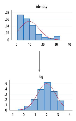
Variables that violate model assumptions will often do so due to high skewness (non symetric distribution)
A possible fix might be to transform the scale on which those variables are measured.
Often:
- logarithmic transformation (predictor will have a quadratic effect on the dependent variable)
- square transformation (more complex to interpret)
Logarithmic coefficients
linear relationship (last week) \[Y = \alpha + \beta X\]
log-linear relationship \[ln Y = \alpha + \beta X\]
lin-log relationship \[Y = \alpha + \beta ln X\]
log-log relationship \[ln Y = \alpha + \beta ln X\]
An increase in 1 unit of \(X\) is associated with an increase of \(\beta\) unit in \(Y\)
An increase in 1 unit of \(X\) is associated with a \(100 \ \beta\%\) change in \(Y\)
A \(1\%\) increase in \(X\) is associated with a \(0.01 \ \beta\%\) change in \(Y\)
A \(1\%\) increase in \(X\) is associated with a \(\beta\%\) change in \(Y\)
Generalized Linear Models (GLM)
Nonlinearity for models
When dealing with a binary dependent variable (\(Y = 0\) or \(Y = 1\)), logistic regression is commonly used.
In logistic regression, we introduce a link function to model the relationship between the predictor(s) and the binary response variable.
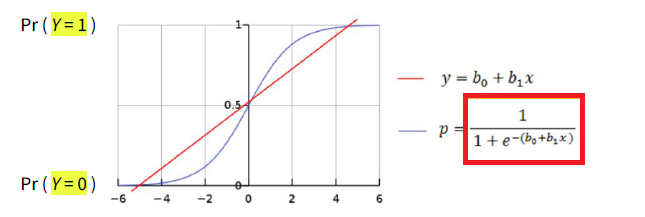
It allows to express the relationship between Y and its predictor(s) through a linear model, at the price of having to interpret that relationship through log-odds, which can be converted into probabilities of \(P(Y = 1)\) through exponentiation (see after).
Logistic regression coefficients
Logistic regression equation
\[L = \underbrace{ln (\frac{p}{1-p})}_\text{= log-odds = logit } = \alpha + \beta X \qquad\text{ or } \qquad p = \frac{e^{\alpha + \beta X}}{1 + e^{\alpha + \beta X}}\]
with
- \(p = P(Y = 1)\)
- \(\ln\) : natural logarithm.
- \(X\) is the predictor variable.
- \(\alpha\) is the intercept.
- \(\beta\) is the coefficient associated with the predictor variable.
Interpretation : odd-ratios
\[\text{Odds Ratio} = e^\beta\]
For 1-unit increase in \(X\), \(P(Y = 1)\) increase by a factor of \(e^\beta\).
- \(OR > 1\) denotes a higher probability of Y = 1 (OR = 1.24 denotes a 24% increase)
- \(OR < 1\) denotes a lower probability of Y = 1 (OR = 0.5 denotes \(P(Y=1)\) divided by 2)
Before Exercise 1
Testing for the presence of the bacterium H. influenzae (y) in children based on the administration of a medication versus a placebo (trt). The presence of the virus was monitored at weeks 0, 2, 4, 6, and 11 (week).
'data.frame':   220 obs. of  6 variables:
 $ y   : Factor w/ 2 levels "n","y": 2 2 2 2 2 2 1 2 2 2 ...
 $ ap  : Factor w/ 2 levels "a","p": 2 2 2 2 1 1 1 1 1 1 ...
 $ hilo: Factor w/ 2 levels "hi","lo": 1 1 1 1 1 1 1 1 2 2 ...
 $ week: int  0 2 4 11 0 2 6 11 0 2 ...
 $ ID  : Factor w/ 50 levels "X01","X02","X03",..: 1 1 1 1 2 2 2 2 3 3 ...
$ trt : Factor w/ 3 levels "placebo","drug",..: 1 1 1 1 3 3 3 3 2 2 ...In mean, bacteria presence decreases with time
              0          1
  0  0.10000000 0.90000000
  2  0.09090909 0.90909091
  4  0.26190476 0.73809524
  6  0.27500000 0.72500000
  11 0.27272727 0.72727273
In mean, bacteria presence decreases thanks to drugs
Fit models (most parsimonious to full).
Note: If you forget to specify family = binomial in the glm function for a binary response variable (i.e., a binary logistic regression), the default family assumed is family = gaussian, which corresponds to linear regression.
Compare them.
=====================================================
                Model 1      Model 2      Model 3
-----------------------------------------------------
(Intercept)        1.41 ***     1.96 ***     2.55 ***
                  (0.17)       (0.29)       (0.41)
week                           -0.11 *      -0.12 **
                               (0.04)       (0.04)
trtdrug                                     -1.11 **
                                            (0.43)
trtdrug+                                    -0.65
                                            (0.45)
-----------------------------------------------------
AIC              219.38       214.91       211.81
BIC              222.77       221.70       225.38
Log Likelihood  -108.69      -105.45      -101.90
Deviance         217.38       210.91       203.81
Num. obs.        220          220          220
=====================================================
*** p < 0.001; ** p < 0.01; * p < 0.05
GLM2 (Model 3) minimizes AIC and seems to be the best model.
Exponentiate GLM2 coefficients to read log-odds.
# A tibble: 4 × 5
  term        estimate std.error statistic  p.value
  <chr>          <dbl>     <dbl>     <dbl>    <dbl>
1 (Intercept)   12.8      0.406       6.28 3.42e-10
2 trtdrug        0.331    0.425      -2.60 9.25e- 3
3 trtdrug+       0.521    0.446      -1.46 1.44e- 1
4 week           0.891    0.0441     -2.62 8.72e- 3
For 1-unit increase in
week, \(P(Y = 1)\) is divided by1/0.89 = 1.12.Taking resp. drug/drug+ instead of a placebo, \(P(Y = 1)\) is divided by 3 and 2.
Exam 2
- Instructions here
- in group & graded (like Exam 1)
- same real-world dataset (road traffic accidents in France)
- data visualisation and data analysis (correlation, link between variables) tasks
- Submit a script called
exam2_solution.R(Subject : “DSR Exam 2 Submission”, To : kim.antunez@sciencespo.fr) - Deadline : apr. 30th, before 7:15 pm.
- Make sure your script is well-organized (you all did well last time)