Spatial 1

Session 11

Kim Antunez & Etienne Côme

2024-04-17

The spatial ecosystem in R.

About the Exams…

Exam 1 (in groups) [coef 33%] : given on feb. 27th for mar. 12th. DONE
Exam 2 (in groups) [coef 33%] : given on apr. 16th for apr. 30th
- Datavisualisation, tests, and linear models.
- Shorter than expected 9 questions => 6 questions
Exam 3 (individual) [coef 33%] : given on apr. 16th for may. 7th
- Part 1: R all by yourself!
- Part 2: reflection upon what you learned during the semester (motivation letter)

Introduction to `sf`

Simple Features for R website.
sf stands for Simple Features.
Its goal is to consolidate the functionality of previous packages (sp, rgeos, and rgdal) into one.
It simplifies the manipulation of spatial data using simple objects.
Compatible with tidy data principles: works well with the tidyverse syntax, including the pipe operator |>.
Main author and maintainer: Edzer Pebesma (also the author of the sp package).

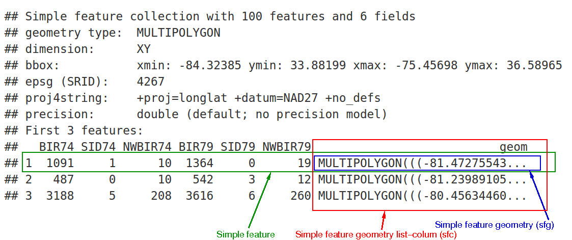
Structure of an `sf` object:

Importing / Exporting Data

Importing:

library(sf)

mtq <- read_sf(paste0(repository, "/martinique.gpkg"))

mtq <- st_read(paste0(repository, "/martinique.gpkg"))

Reading layer `martinique' from data source 
  `https://minio.lab.sspcloud.fr/kantunez/diffusion/dsr/martinique.gpkg' 
  using driver `GPKG'
Simple feature collection with 34 features and 23 fields
Geometry type: POLYGON
Dimension:     XY
Bounding box:  xmin: 690574.4 ymin: 1592426 xmax: 736126.5 ymax: 1645660
Projected CRS: WGS 84 / UTM zone 20N

Exporting

# Export
write_sf(mtq, "data/mtq/martinique.gpkg", delete_layer = TRUE)
st_write(mtq, "data/mtq/martinique.gpkg", delete_layer = TRUE)

The GeoPackage (gpkg) format is an open format (not tied to an operating system) and implemented as a SQLite database.

Also note the existence of the GeoParquet format, extremely efficient for processing large volumes of spatial data.

Coordinate System

Coordinate systems/projections are identified using a code called an EPSG code:

lat/long : 4326 https://epsg.io/4326
Lambert 93 : 2154 https://epsg.io/2154
Pseudo-Mercator : 3857 https://epsg.io/3857
Lambert azimuthal equal area : 3035 https://epsg.io/3035

Projection

Obtain the projection using st_crs() (epsg code) and modify it using st_transform().

sf uses spherical geometry by default for unprojected data since version 1.0, thanks to the s2 library. See https://r-spatial.github.io for more details.

st_crs(mtq)

Coordinate Reference System:
  User input: WGS 84 / UTM zone 20N 
  wkt:
PROJCRS["WGS 84 / UTM zone 20N",
    BASEGEOGCRS["WGS 84",
        ENSEMBLE["World Geodetic System 1984 ensemble",
            MEMBER["World Geodetic System 1984 (Transit)"],
            MEMBER["World Geodetic System 1984 (G730)"],
            MEMBER["World Geodetic System 1984 (G873)"],
            MEMBER["World Geodetic System 1984 (G1150)"],
            MEMBER["World Geodetic System 1984 (G1674)"],
            MEMBER["World Geodetic System 1984 (G1762)"],
            MEMBER["World Geodetic System 1984 (G2139)"],
            ELLIPSOID["WGS 84",6378137,298.257223563,
                LENGTHUNIT["metre",1]],
            ENSEMBLEACCURACY[2.0]],
        PRIMEM["Greenwich",0,
            ANGLEUNIT["degree",0.0174532925199433]],
        ID["EPSG",4326]],
    CONVERSION["UTM zone 20N",
        METHOD["Transverse Mercator",
            ID["EPSG",9807]],
        PARAMETER["Latitude of natural origin",0,
            ANGLEUNIT["degree",0.0174532925199433],
            ID["EPSG",8801]],
        PARAMETER["Longitude of natural origin",-63,
            ANGLEUNIT["degree",0.0174532925199433],
            ID["EPSG",8802]],
        PARAMETER["Scale factor at natural origin",0.9996,
            SCALEUNIT["unity",1],
            ID["EPSG",8805]],
        PARAMETER["False easting",500000,
            LENGTHUNIT["metre",1],
            ID["EPSG",8806]],
        PARAMETER["False northing",0,
            LENGTHUNIT["metre",1],
            ID["EPSG",8807]]],
    CS[Cartesian,2],
        AXIS["(E)",east,
            ORDER[1],
            LENGTHUNIT["metre",1]],
        AXIS["(N)",north,
            ORDER[2],
            LENGTHUNIT["metre",1]],
    USAGE[
        SCOPE["Engineering survey, topographic mapping."],
        AREA["Between 66°W and 60°W, northern hemisphere between equator and 84°N, onshore and offshore. Anguilla. Antigua and Barbuda. Bermuda. Brazil. British Virgin Islands. Canada - New Brunswick; Labrador; Nova Scotia; Nunavut; Prince Edward Island; Quebec. Dominica. Greenland. Grenada. Guadeloupe. Guyana. Martinique. Montserrat. Puerto Rico. St Kitts and Nevis. St Barthelemy. St Lucia. St Maarten, St Martin. St Vincent and the Grenadines. Trinidad and Tobago. Venezuela. US Virgin Islands."],
        BBOX[0,-66,84,-60]],
    ID["EPSG",32620]]

mtq_4326 <- mtq |> st_transform(4326)

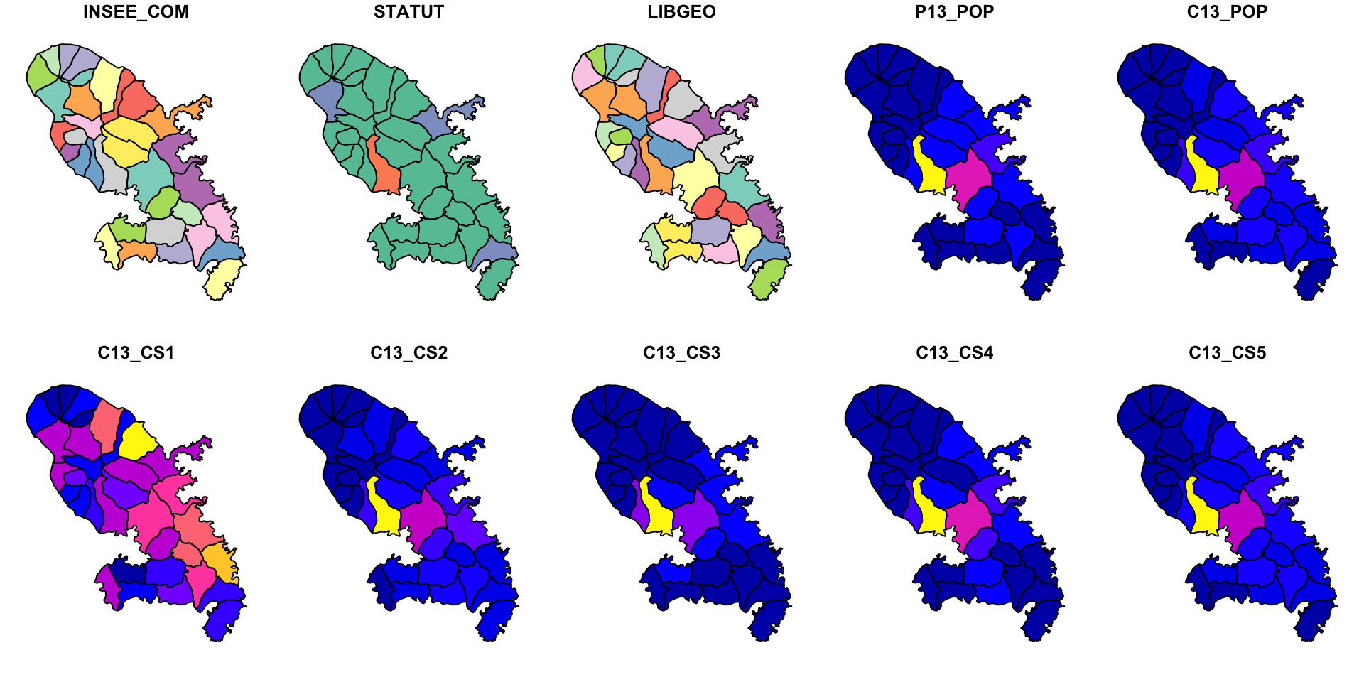
Displaying data

Default display:

plot(mtq)

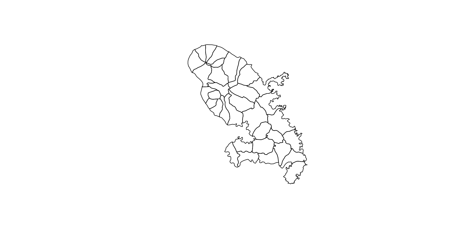
Keep only the geometry:

plot(st_geometry(mtq))

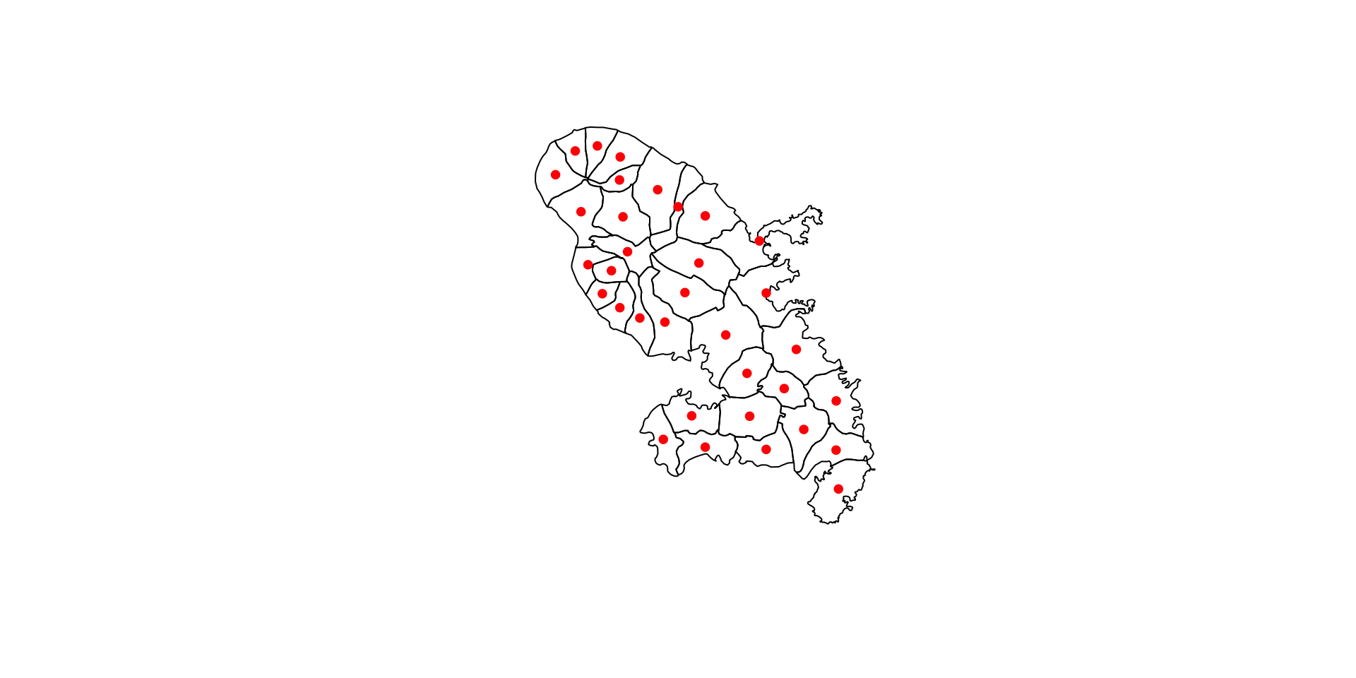
Extract Centroids

mtq_c <- st_centroid(mtq) 
plot(st_geometry(mtq))
plot(st_geometry(mtq_c), add = TRUE, cex = 1.2, col = "red", pch = 20)

Distance Matrix

mat <- st_distance(x = mtq_c, y = mtq_c)
mat[1:5, 1:5]

Units: [m]
          [,1]     [,2]      [,3]      [,4]      [,5]
[1,]     0.000 35297.56  3091.501 12131.617 17136.310
[2,] 35297.557     0.00 38332.602 25518.913 18605.249
[3,]  3091.501 38332.60     0.000 15094.702 20226.198
[4,] 12131.617 25518.91 15094.702     0.000  7177.011
[5,] 17136.310 18605.25 20226.198  7177.011     0.000

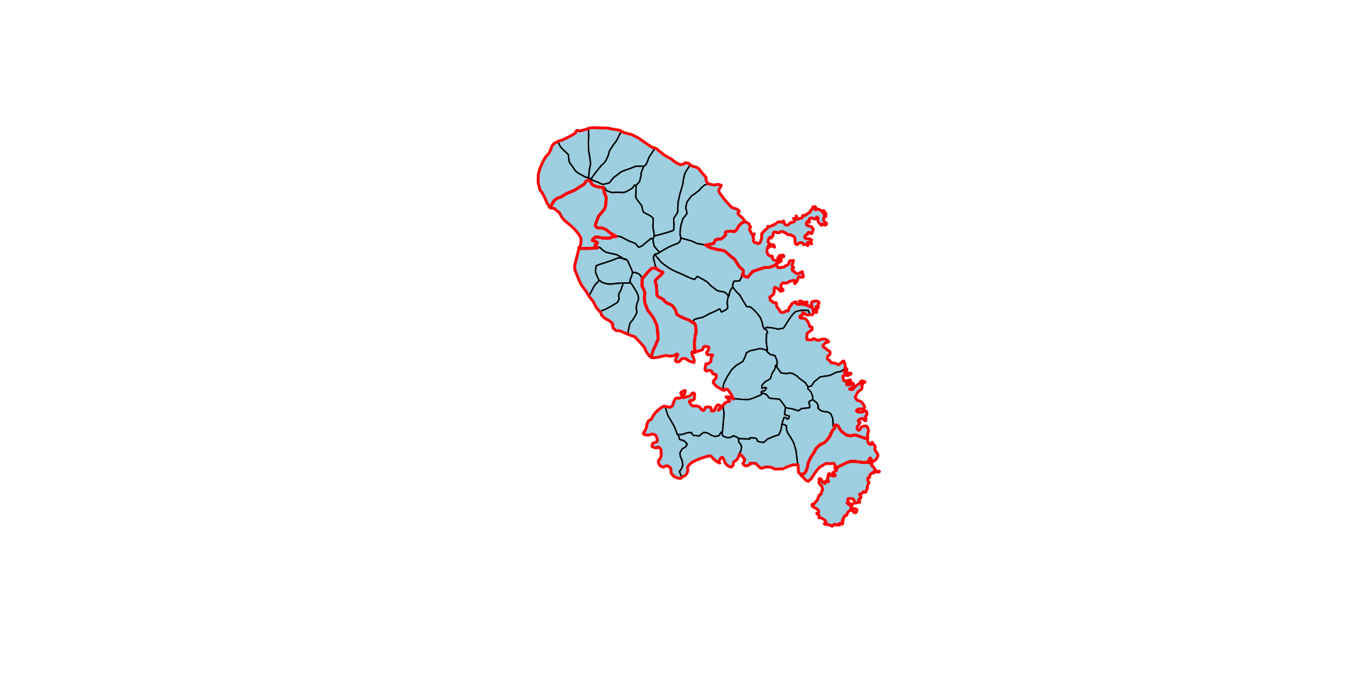
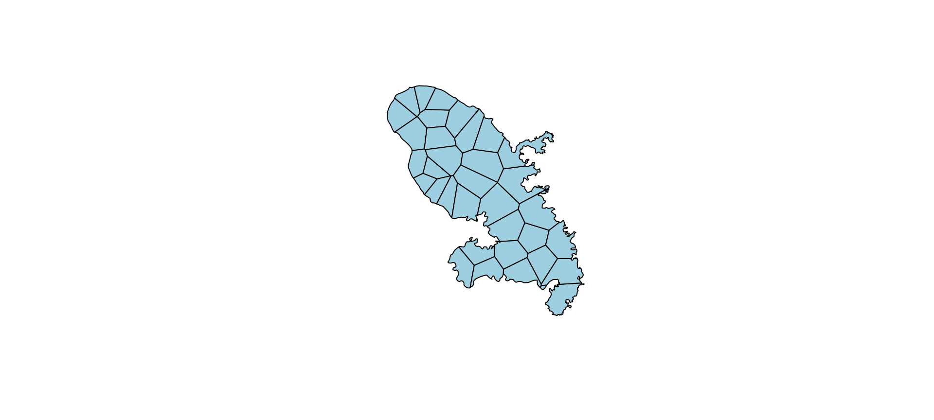
Polygon Aggregation

Simple union:

mtq_u <- st_union(mtq)
plot(st_geometry(mtq), col="lightblue")
plot(st_geometry(mtq_u), add=T, lwd=2, border = "red")

Using a grouping variable:

library(dplyr)
mtq_u2 <- mtq |> 
  group_by(STATUT) |> 
  summarize(P13_POP = sum(P13_POP))
plot(st_geometry(mtq), col="lightblue")
plot(st_geometry(mtq_u2), add = TRUE, lwd = 2, border = "red", col = NA)

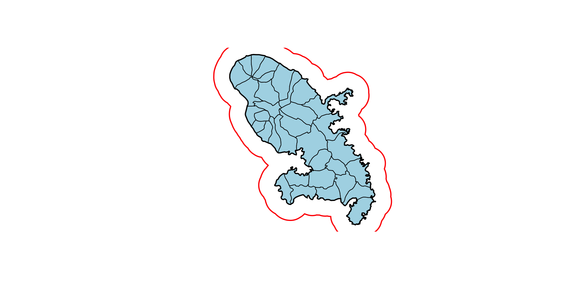
Buffer Zone

mtq_b <- st_buffer(x = mtq_u, dist = 5000)
plot(st_geometry(mtq), col = "lightblue")
plot(st_geometry(mtq_u), add = TRUE, lwd = 2)
plot(st_geometry(mtq_b), add = TRUE, lwd = 2, border = "red")

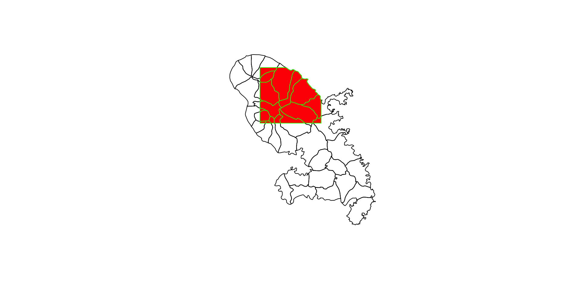
Polygon Intersection

Creating a polygon.

m <- rbind(c(700015,1624212), c(700015,1641586), c(719127,1641586), 
           c(719127,1624212), c(700015,1624212))
p <- st_sf(st_sfc(st_polygon(list(m))), crs = st_crs(mtq))
plot(st_geometry(mtq))
plot(p, border = "red", lwd = 2, add = TRUE)

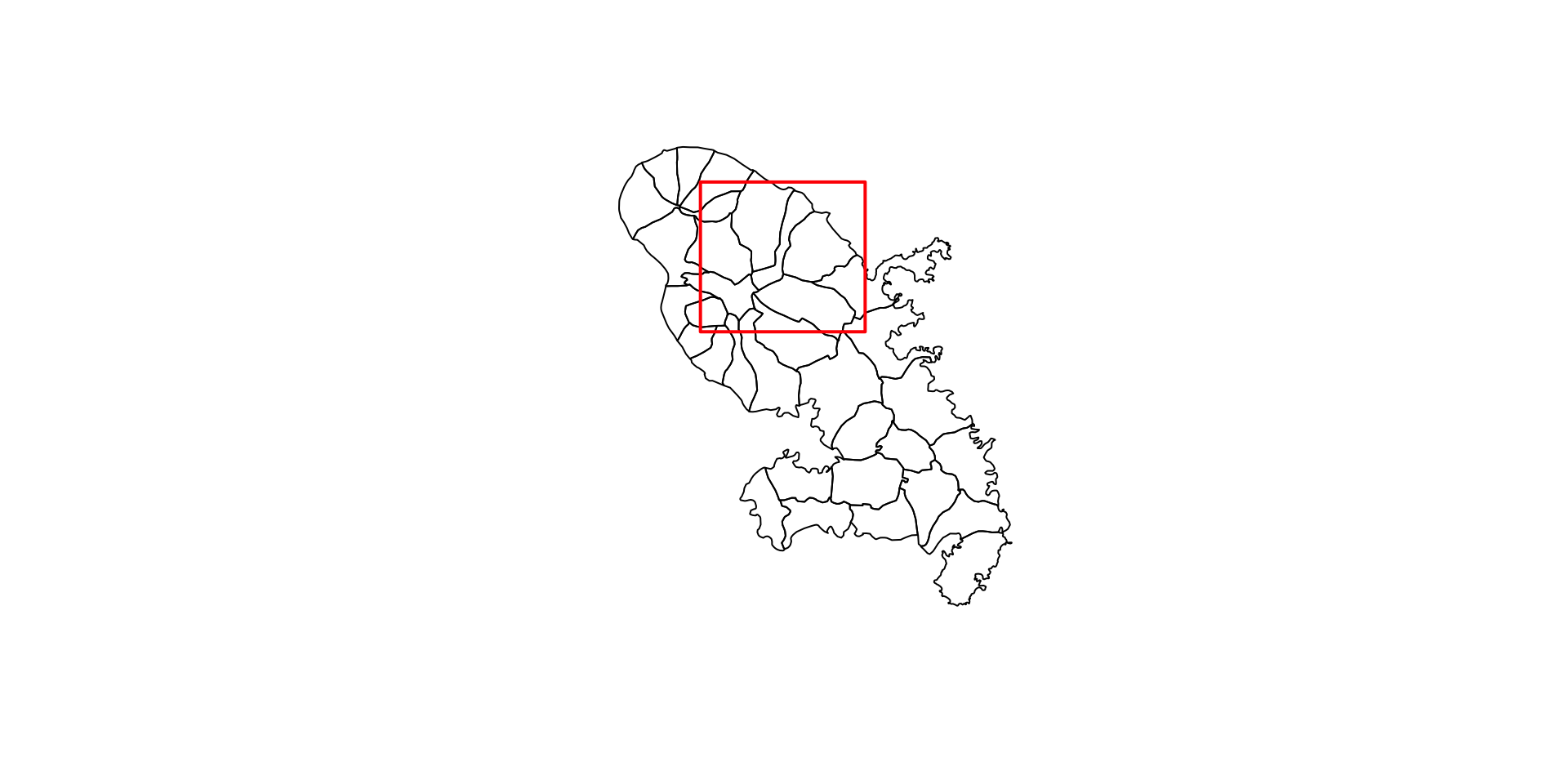
st_intersection() extracts the part of mtq that intersects with the created polygon.

mtq_z <- st_intersection(x = mtq, y = p)
plot(st_geometry(mtq))
plot(st_geometry(mtq_z), col = "red", border = "green", add = TRUE)

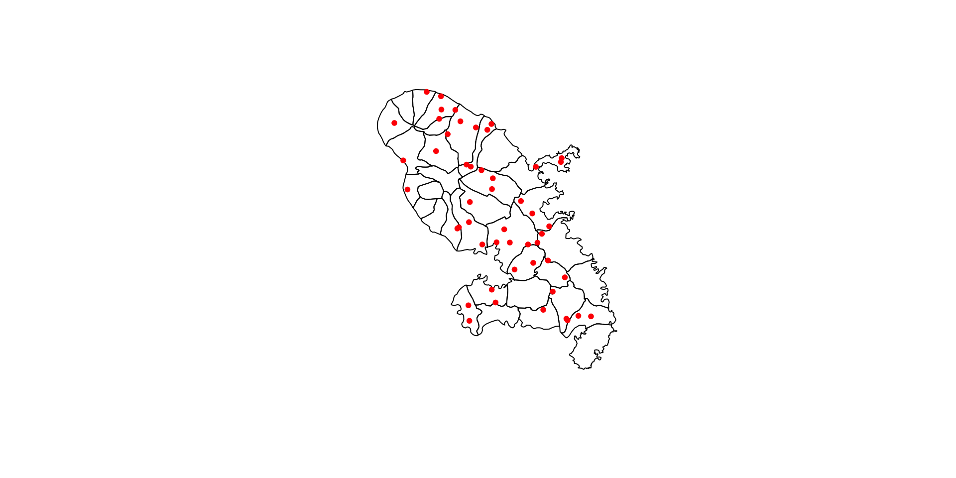
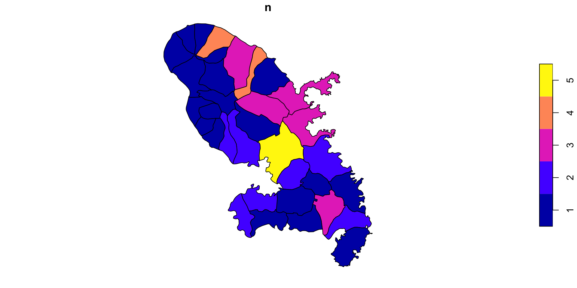
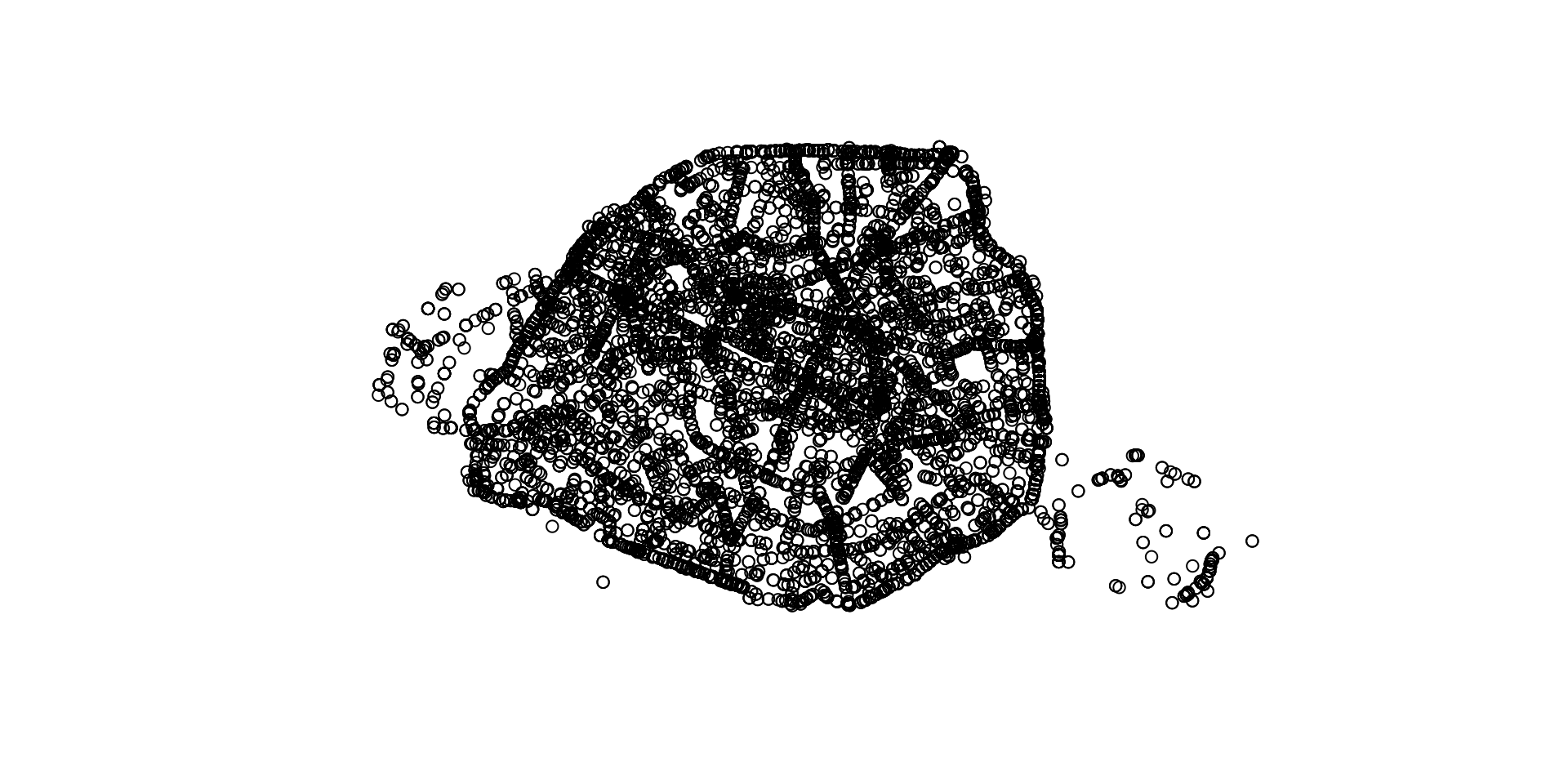
Counting Points in Polygons

st_sample() creates random points on the map.

pts <- st_sample(x = mtq, size = 50)
plot(st_geometry(mtq))
plot(pts, pch = 20, col = "red", add=TRUE, cex = 1)

st_join performs a spatial join coupled with aggregation.

It is possible to finely control the join (points on boundaries, etc.) with the join argument, which defaults to st_intersects(). See here for a precise definition of possible spatial predicates.

mtq_counts <- mtq |>
st_join(st_as_sf(pts))

head(mtq_counts |> select(INSEE_COM),3)

Simple feature collection with 3 features and 1 field
Geometry type: POLYGON
Dimension:     XY
Bounding box:  xmin: 697601.7 ymin: 1598817 xmax: 710461.9 ymax: 1640521
Projected CRS: WGS 84 / UTM zone 20N
    INSEE_COM                           geom
1       97201 POLYGON ((699261.2 1637681,...
2       97202 POLYGON ((709840 1599026, 7...
2.1     97202 POLYGON ((709840 1599026, 7...

mtq_counts <- mtq_counts |>
count(INSEE_COM)

head(mtq_counts)

Simple feature collection with 6 features and 2 fields
Geometry type: POLYGON
Dimension:     XY
Bounding box:  xmin: 695444.4 ymin: 1598817 xmax: 717731.2 ymax: 1645182
Projected CRS: WGS 84 / UTM zone 20N
  INSEE_COM n                           geom
1     97201 1 POLYGON ((699261.2 1637681,...
2     97202 2 POLYGON ((709840 1599026, 7...
3     97203 4 POLYGON ((706092.8 1642964,...
4     97204 1 POLYGON ((697314.8 1623213,...
5     97205 1 POLYGON ((702756.8 1617978,...
6     97206 1 POLYGON ((709840 1599026, 7...

plot(mtq_counts|> select(n))
plot(pts, pch = 20, col = "red", add = TRUE, cex = 1)

Voronoi Polygons

A Voronoi diagram is a plane partitioning into cells (adjacent regions, called Voronoi polygons) based on a discrete set of points. Each cell encloses a single point and forms the set of points in the plane that are closer to that point than to any other.

Also, see here and here.

mtq_v <- st_collection_extract(st_voronoi(x = st_union(mtq_c)))
mtq_v <- st_intersection(mtq_v, st_union(mtq))
mtq_v <- st_join(x = st_sf(mtq_v), y = mtq_c)
plot(st_geometry(mtq_v), col='lightblue')

Other operations

st_area(x)
st_length(x)
st_disjoint(x, y, sparse = FALSE)
st_touches(x, y, sparse = FALSE)
st_crosses(s, s, sparse = FALSE)
st_within(x, y, sparse = FALSE)
st_contains(x, y, sparse = FALSE)

st_overlaps(x, y, sparse = FALSE)
st_equals(x, y, sparse = FALSE)
st_covers(x, y, sparse = FALSE)
st_covered_by(x, y, sparse = FALSE)
st_equals_exact(x, y,0.001, sparse = FALSE)
…

Conversion

st_cast
st_collection_extract
st_sf
st_as_sf
st_as_sfc

Creating Interactive and Static Maps

In this section, we will visualize data on personal injury road traffic accidents in 2019.

This is a data.frame containing two columns, providing information about the latitude and longitude of road accidents.

accidents.2019.paris <- readRDS(paste0(repository,"/accidents2019_paris.RDS"))
head(accidents.2019.paris)

# A tibble: 6 × 13
     Num_Acc id_vehicule  grav sexe  an_nais   lat  long com   int   lum   voie 
       <dbl> <chr>       <dbl> <fct>   <dbl> <dbl> <dbl> <chr> <fct> <fct> <chr>
1    2.02e11 138 305 660     1 Fémi…    1983  48.9  2.28 75117 Inte… Nuit… BD P…
2    2.02e11 138 305 661     4 Masc…    1975  48.9  2.28 75117 Inte… Nuit… BD P…
3    2.02e11 138 305 658     4 Fémi…    1988  48.8  2.41 75120 Inte… Nuit… COUR…
4    2.02e11 138 305 658     1 Masc…    1991  48.8  2.41 75120 Inte… Nuit… COUR…
5    2.02e11 138 305 658     4 Masc…    1987  48.8  2.41 75120 Inte… Nuit… COUR…
6    2.02e11 138 305 659     1 Masc…    1996  48.8  2.41 75120 Inte… Nuit… COUR…
# ℹ 2 more variables: catr <fct>, catv <fct>

We need to convert this data.frame into a spatial object (sf) using the st_as_sf function. Simply specify the column names containing the coordinates and the projection, here CRS = 4326 (WGS 84). We then transform this data into CRS = 2154 (Lambert 93).

accidents.2019.paris <- st_as_sf(accidents.2019.paris,
                                coords = c("long", "lat"),
                                crs = 4326) |>
  st_transform(2154)

plot(st_geometry(accidents.2019.paris))

Interactive Maps

Several solutions exist for creating interactive maps with R. mapview, leaflet and mapdeck are the main ones. For simplicity, we focus here on mapview.

Interactive maps are not necessarily very relevant for representing geostatistical information. However, they are useful for exploring databases. Let’s see an example with mapview regarding fatal accidents in Paris in 2019.

library(mapview)

individus_tues <- accidents.2019.paris |>
  filter(grav == 2) |> # grav = 2 : individus tués
  mutate(age=2019-an_nais) # age
mapview(individus_tues)

When you click on a point, the values of various variables in the database appear. This can help in exploring the database. Let’s customize a bit….

mapview(individus_tues,
        legend = TRUE, #map.types = "Stamen.TonerLite",
        cex = 5, col.regions = "#217844", lwd = 0, alpha = 0.9,
        layer.name = 'Individus tués')

Let’s customize a bit more…

However, adding a legend for the size of proportional circles is not easily done.

mapview(individus_tues,
       legend=TRUE, # map.types = "Stamen.TonerLite", 
        layer.name = 'Individus tués',
        cex="age", zcol="sexe", lwd=0, alpha=0.9
       )

Static Maps with `ggplot2`

Once again, various R packages are used to create static maps:

ggplot2 is a widely used package for various types of plots and has been specifically adapted for maps (geom_sf).
The tmap package contains advanced functionalities based on the logic of ggplot2.
mapsf (successor of cartography) relies on a so-called “base R” language and allows for basic as well as advanced cartographic representations.

For simplicity’s sake, we’ll concentrate here on ggplot2, a well-known package for all types of graphics.

Grammar of Graphics

Wilkinson, L., Anand, A., & Grossman, R. (2005). Graph-theoretic scagnostics. In Information Visualization, IEEE Symposium on (pp. 21-21). IEEE Computer Society.
Adopted by Wickham, H. (2010). A layered grammar of graphics. Journal of Computational and Graphical Statistics, 19(1), 3-28. And implemented in ggplot2.
Grammar → same type of construction/philosophy for all types of plots

Components of the Grammar

Data and Aesthetic Characteristics (aes)

e.g., f(data) → x position, y position, size, shape, color

Geometric Objects

e.g., points, lines, bars, texts

Scales (scales)

e.g., f([0, 100]) → [0, 5] px

Specification of Components (facet)

e.g., Segmentation of data based on one or more factors

Statistical Transformation

e.g., mean, count, regression…

The Coordinate System

Integrating Spatial Data with `geom_sf`

A brief introduction/reminder of graphic semiology:

We are working with the cartographic layer of IRIS¹.

library(sf)
library(dplyr)
iris.75 <- st_read(paste0(repository, "/iris_75.gpkg"), stringsAsFactors = F)

Reading layer `iris_75' from data source 
  `https://minio.lab.sspcloud.fr/kantunez/diffusion/dsr/iris_75.gpkg' 
  using driver `GPKG'
Simple feature collection with 992 features and 2 fields
Geometry type: MULTIPOLYGON
Dimension:     XY
Bounding box:  xmin: 643075.6 ymin: 6857477 xmax: 661086.2 ymax: 6867081
Projected CRS: RGF93 v1 / Lambert-93

Let’s count the number of people injured (nbacc) per IRIS:

acc_iris <- iris.75 |> st_join(accidents.2019.paris) |> 
  group_by(CODE_IRIS) |> dplyr::summarize(nb_acc = n(),
            nb_acc_grav = sum(if_else(grav%in%c(2,3), 1, 0),
                        na.rm = TRUE),
            nb_vl = sum(if_else(catv == "VL seul", 1, 0),
                        na.rm = TRUE),
            nb_edp = sum(if_else(catv == "EDP à moteur", 1, 0),
                         na.rm = TRUE),
            nb_velo = sum(if_else(catv == "Bicyclette", 1, 0),
                          na.rm = TRUE)
            ) 
head(acc_iris,1)

Simple feature collection with 1 feature and 6 fields
Geometry type: MULTIPOLYGON
Dimension:     XY
Bounding box:  xmin: 651771.6 ymin: 6862103 xmax: 652179 ymax: 6862406
Projected CRS: RGF93 v1 / Lambert-93
# A tibble: 1 × 7
  CODE_IRIS nb_acc nb_acc_grav nb_vl nb_edp nb_velo                         geom
  <chr>      <int>       <dbl> <dbl>  <dbl>   <dbl>           <MULTIPOLYGON [m]>
1 751010101     27           1    11      1       4 (((652130.3 6862122, 652126…

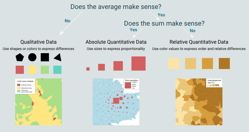
Maps with Proportional Circles

Code

library(ggplot2)
ggplot() +
  geom_sf(data = acc_iris, colour = "ivory3", fill = "ivory") +
  geom_sf(data = acc_iris |>  st_centroid(),
          aes(size= nb_acc), colour="#E84923CC", show.legend = 'point') +
  scale_size(name = "Nombre d'accidents",
             breaks = c(1,10,100,200),
             range = c(0,5)) +
   coord_sf(crs = 2154, datum = NA,
            xlim = st_bbox(iris.75)[c(1,3)],
            ylim = st_bbox(iris.75)[c(2,4)]) +
  theme_minimal() +
  theme(panel.background = element_rect(fill = "ivory",color=NA),
        plot.background = element_rect(fill = "ivory",color=NA),legend.position = "bottom") +
  labs(title = "Nombre d'accidents de la route à Paris par iris",
       caption = "fichier BAAC 2019, ONISR\nantuki & comeetie, 2023",x="",y="")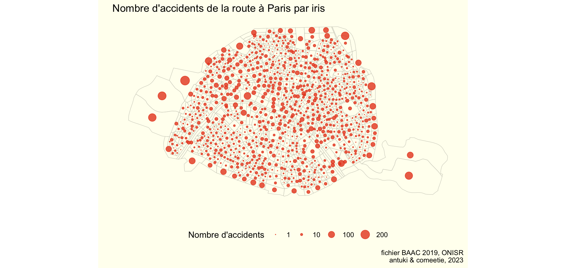

Choropleth Maps

Code

library(RColorBrewer) #pour les couleurs des palettes
# Quintiles de la part des accidents ayant eu lieu à vélo
perc_velo = 100*acc_iris$nb_velo/acc_iris$nb_acc
bks <- c(0,round(quantile(perc_velo[perc_velo!=0],na.rm=TRUE,probs=seq(0,1,0.25)),1))
# Intégration dans la base de données
acc_iris <- acc_iris |> mutate(txaccvelo = 100*nb_velo/nb_acc,
                     txaccvelo_cat = cut(txaccvelo,bks,include.lowest = TRUE)) 

# Carte
ggplot() +
  geom_sf(data = iris.75,colour = "ivory3",fill = "ivory") +
  geom_sf(data = acc_iris, aes(fill = txaccvelo_cat)) +
  scale_fill_brewer(name = "Part (En %)",
                    palette = "Reds",
                    na.value = "grey80") +
  coord_sf(crs = 2154, datum = NA,
           xlim = st_bbox(iris.75)[c(1,3)],
           ylim = st_bbox(iris.75)[c(2,4)]) +
  theme_minimal() +
  theme(panel.background = element_rect(fill = "ivory",color=NA),
        plot.background = element_rect(fill = "ivory",color=NA),legend.position="bottom") +
  labs(title = "Part des accidentés à vélos",
       subtitle = "par arrondissement à Paris en 2019",
       caption = "fichier BAAC 2019, ONISR\nantuki & comeetie, 2023",
       x = "", y = "")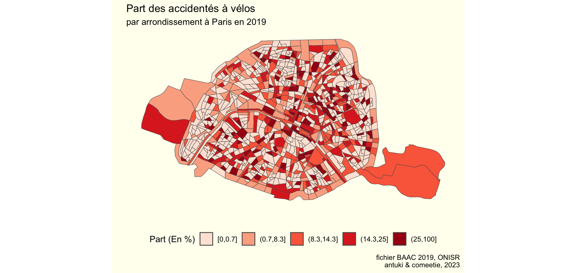

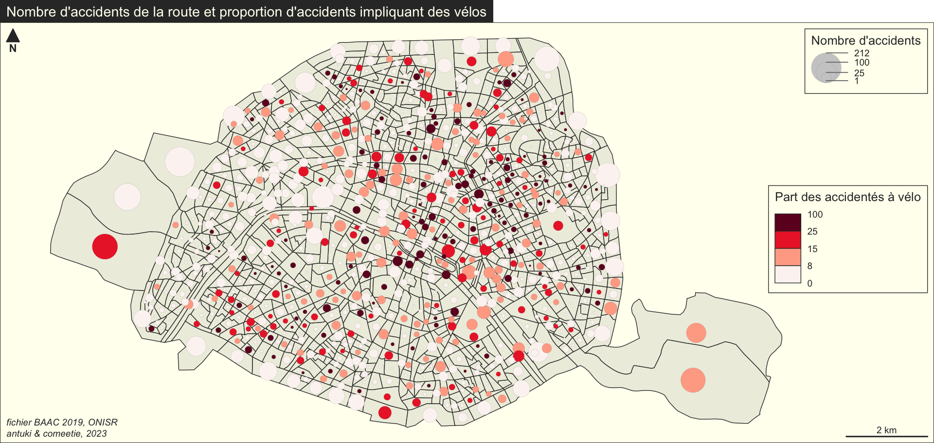
Maps with `mapsf`

Below is an example of a similar map created using the mapsf library syntax.

Code

library(mapsf)
mf_theme("default",cex=0.9,mar=c(0,0,1.2,0),bg="ivory")
mf_init(x = acc_iris, expandBB = c(0, 0, 0, .15)) 
mf_map(acc_iris,add = TRUE,col = "ivory2")
# Plot symbols with choropleth coloration
mf_map(
  x = acc_iris |>  st_centroid(),
  var = c("nb_acc", "txaccvelo"),
  type = "prop_choro",
  border = "grey50",
  lwd = 0.1,
  leg_pos = c("topright","right"),
  leg_title = c("Nombre d'accidents", "Part des accidentés à vélo"),
  breaks = c(0,8,15,25,100),
  nbreaks = 5,
  inches= 0.16,
  pal = "Reds",
  leg_val_rnd = c(0, 0),
  leg_frame = c(TRUE, TRUE)
)
mf_layout(
  title = "Nombre d'accidents de la route et proportion d'accidents impliquant des vélos",
  credits = "fichier BAAC 2019, ONISR\nantuki & comeetie, 2023",
  frame = TRUE)

Homework for next week

Catch up!
Work on your graded exam
Handbooks, videos, cheatsheets
- session 10: 2 chapters of Hank’s handbook
- session 11: 2 chapters of Baumer’s handbook

Spatial 1

The spatial ecosystem in R.

About the Exams…

Introduction to sf

Structure of an sf object:

Importing / Exporting Data

Coordinate System

Projection

Displaying data

Extract Centroids

Distance Matrix

Polygon Aggregation

Buffer Zone

Polygon Intersection

Counting Points in Polygons

Voronoi Polygons

Other operations

Conversion

Creating Interactive and Static Maps

Interactive Maps

Static Maps with ggplot2

Grammar of Graphics

Integrating Spatial Data with geom_sf

Maps with Proportional Circles

Choropleth Maps

Maps with mapsf

Homework for next week

Introduction to `sf`

Structure of an `sf` object:

Static Maps with `ggplot2`

Integrating Spatial Data with `geom_sf`

Maps with `mapsf`