getwd() #To know your working directory
setwd("C:/Desktop/DSR/Session 2") # To set your WD2 Workflow
Session 2
By the end of this session, you have learned how to understand the nature of R code, which outlines a sequence of instructions, by giving basic examples.
In a nutshell
- Importing a CSV dataset into R using the
read.csvfunction (and the same withreadxl::read_excelfor xls files) - Describing a dataset using the
View,strandnrowfunctions to understand its structure. - Selecting specific variables and values from a dataset.
- Using R pipes (
%>%) to chain operations together, providing a more readable and concise code structure. - Creating basic point and line plots with
ggplot2 - Count the values of the categorical variable with
tableand describe continuous ones withsummary - Getting to know
dplyrfunctions such asselectandgroup_by+summarise - Understanding that the output in R includes not only results but also messages, warnings, and errors.
2.1 Essential R syntax to do things
2.1.1 Working directory
By setting the working directory, you specify the location where RStudio will look for files and save outputs.
Using R:
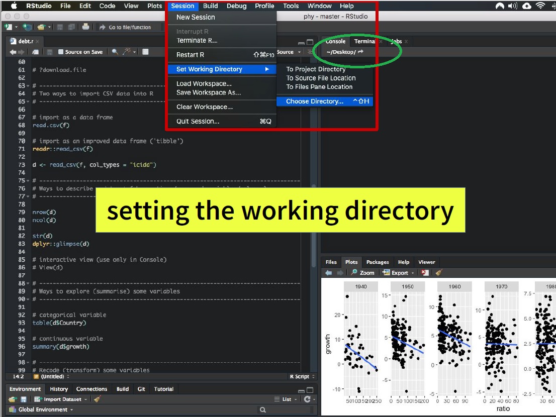
This can be helpful for organizing your projects and ensuring that R scripts can access the necessary files.
To set the working directory in RStudio using the menu, follow these steps:
- Go to the “Session” menu located at the top of the RStudio window.
- Click on “Set Working Directory.”
- From the dropdown menu that appears, select “Choose Directory.” A file dialog will open, allowing you to browse and select the directory you want to set as your working directory.
- click the “Open” button.
You’ll see the path to the chosen directory displayed in the Console panel at the bottom left corner of the RStudio interface or at the top right like in the image.
2.1.2 Exercises
Let’s start with Exercises 1 and Exercise 2 !
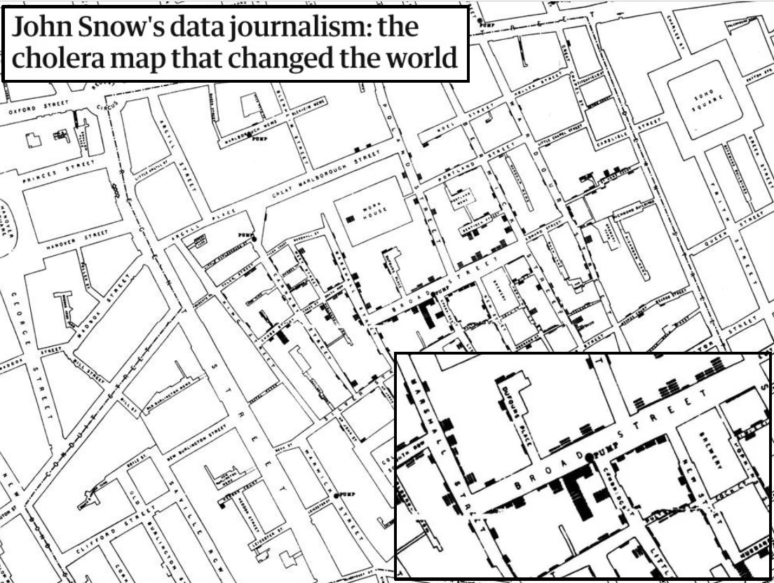
It is Dr. John Snow’s famous map of the 1854 cholera outbreak in Soho, London. He drew and published to document the data collected during the epidemic. Each cross (bold lines stacked along the street) indicates a cholera-related death at that address. The article examines the true story behind the map but overall, it sheds light on the actual role of the map in understanding cholera transmission.
2.1.3 Recap
# import dataset.csv into object data
# [!] set the working directory first
data <- read.csv("data/dataset.csv")

# Describe the dataset
str(data)

# select a variable in a data frame
data$variable

# select values 2 to 5 in a variable
data$variable[2:5]

# select positive values
data$variable[ data$variable > 0]
Syntactic sugar: R pipes (see Irizarry ch. 4.5)
# do what the first line says, and then do
# what the second line says to that result
group_by(data, variable) %>%
summarise(mu_x = mean(x, na.rm = TRUE))

# alternative pipe symbol (base R)
group_by(data, variable) |>
summarise(mu_x = mean(x, na.rm = TRUE))
2.2 Go further
2.2.1 Important principles
- Code is like a cooking recipe — it contains instructions and comments to replicate the results of an analysis
- R code is imperative: ʻdo this, then do that, then that,…ʼ
- Run code from top to bottom: respect order of execution
- Some { blocks of code } or functions span over multiple lines
- Output = results, but also messages, warnings and errors
2.2.2 Useful keyboard shortcuts
Execute / run selected code
Select multiple lines of code
Clear (erase) the Console
Insert <- in your code
Insert %>% in your code
Ctrl/Cmd-Enter
Shift + arrows
Ctrl-L
Alt-dash (Alt + dash ʻ-ʼ key)
Ctrl/Cmd-Shift-M
Ctrl is for Windows and Mac, Cmd for Mac only
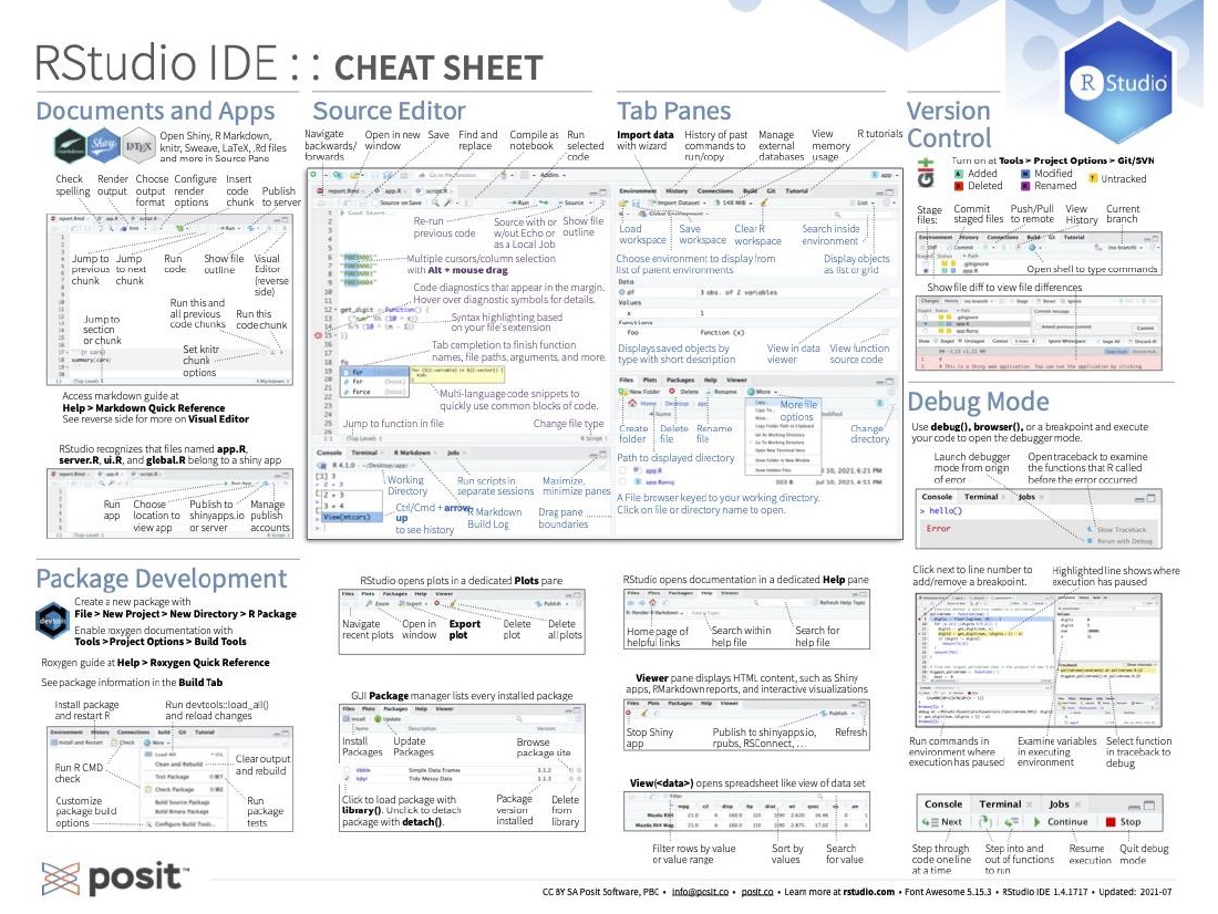
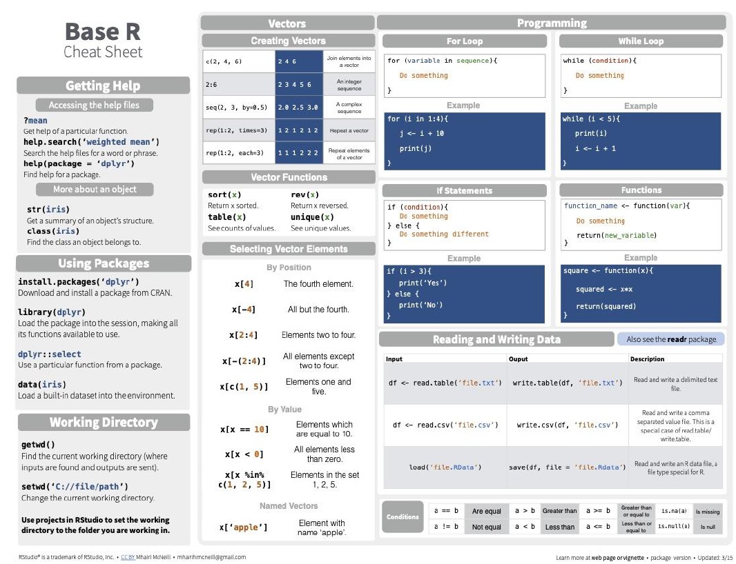
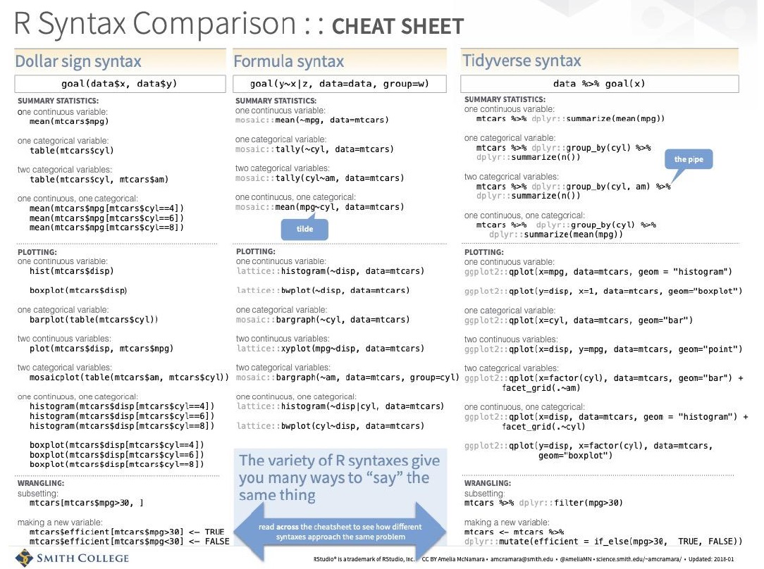
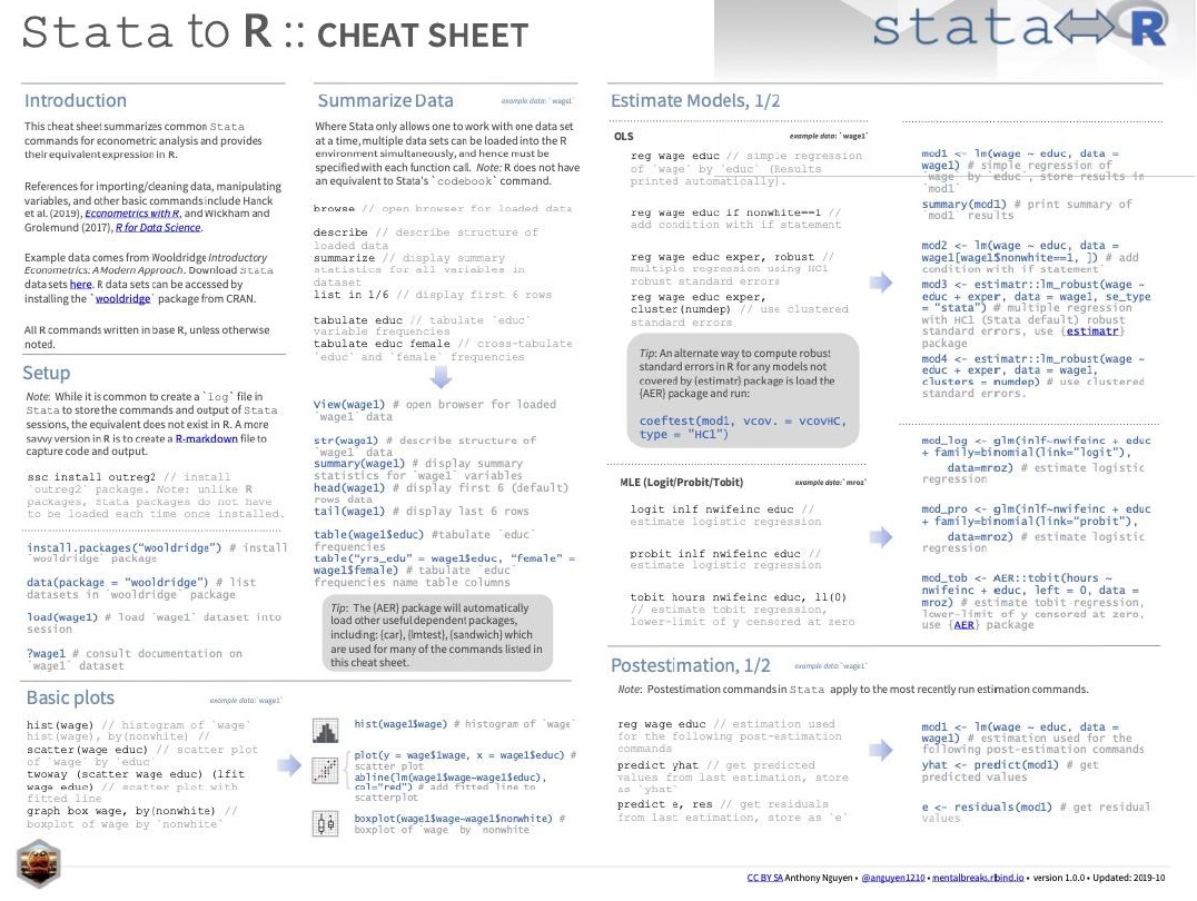
2.2.3 Cheatsheets
Homework for next week
- Finish Exercise 2
- 1 preparation exercise (in group & ungraded, for now)
- Handbooks, videos, cheatsheets
- 3 chapters of Irizarry’s handbook
- 2 chapters of Rodrigues’s handbook
- 1 video
- 2 compulsory Cheatsheets
