Univariate Exploratory analysis

Session 6

François Briatte
(small modifs by Kim Antunez & ChatGPT)

2024-03-12

Exploratory Analysis

Definition

Exploratory analysis is the process of summarizing multiple values of one or more variables using a set of concise summary statistics. It provides an initial understanding of the data, aiding in decision-making, hypothesis generation, and identifying potential outliers or anomalies.

Purpose

It aims to uncover patterns, insights, and key characteristics in the data, helping to understand the underlying structure and relationships:

Descriptive Statistics (Numbers): Measures of central tendency (mean, median, mode) and dispersion (range, variance, standard deviation).
Distributions (Plots): Histograms and density curves.

Distributions

This section introduces the concept of distributions in statistics. A distribution refers to the way data values are spread out or organized. It’s a fundamental concept for understanding the characteristics of data and making informed decisions based on it.

Descriptive statistics (numbers)

Descriptive statistics are numerical measures that provide insight into the central tendency and variability of a dataset.

Measures of Central Tendency:

Mean: The arithmetic average of all data points in a dataset.
Median: The middle value in a sorted dataset; it separates the data into two equal halves. The same goes to other quantiles
Mode: The most frequently occurring value in a dataset.

Measures of Dispersion:

Range: The difference between the maximum and minimum values in a dataset.
Variance: A measure of how much the values in a dataset vary from the mean.
Standard Deviation: The square root of the variance; it provides a standardized measure of data spread.

Distributions (plots)

There are many visual representations of distributions using plots.

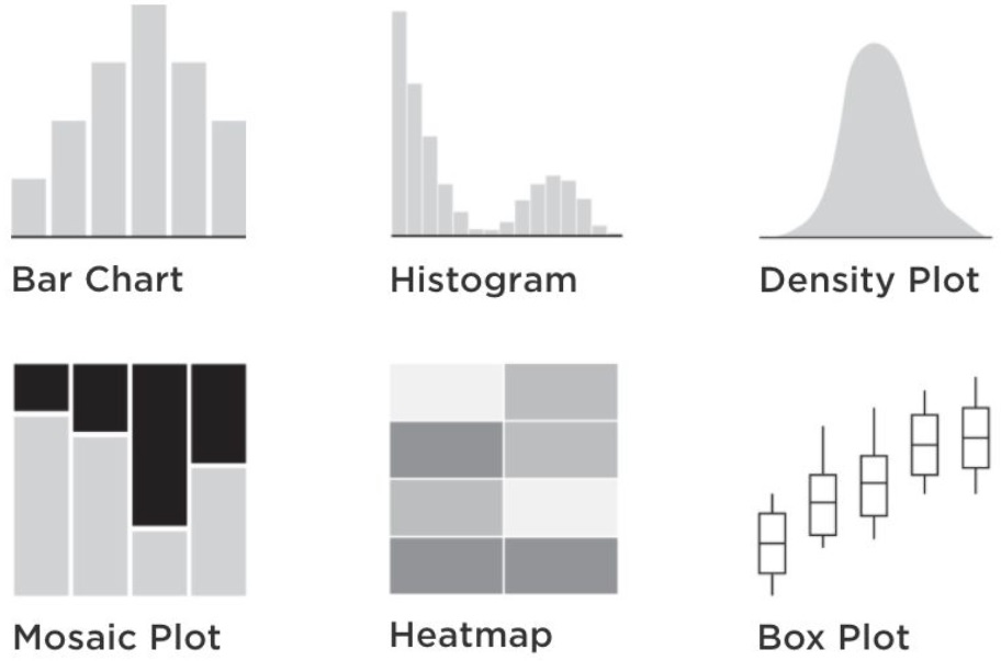
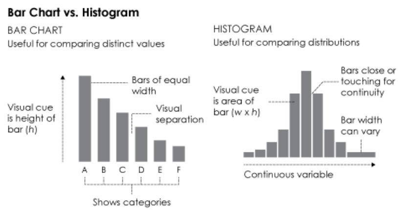
Histograms: A graphical representation of the frequency distribution of data. It divides the data into intervals (bins) and displays the number of data points in each bin. Histograms help understand the shape and spread of data.
Density Curves: A smoothed representation of the distribution of data. It provides insights into the probability density function of continuous data. Density curves are often used to approximate the shape of distributions.

Before Exercise 1

Quantitative / Continuous variables

Quantiles:

x <- rnorm(100)# Extremes & Quartiles by default
x[1:10]

 [1] -0.01879769  0.29734468 -0.72161879  0.81348481 -0.58172615 -0.05933099
 [7]  0.32264855  0.54180014  1.63311884  1.80059136

quantile(x,  probs = c(0.25, 0.5, 0.75))

       25%        50%        75% 
-0.7437115  0.1055856  0.7417393

median(x)

[1] 0.1055856

More about distributions:

range(x)

[1] -3.104271  2.685660

var(x)

[1] 1.192242

sd(x)

[1] 1.091898

Qualitative / Categorical variables

Factors:

x <- c("Animal 2", "Animal 1", "Animal 2", "Animal 3")
as.factor(x)

[1] Animal 2 Animal 1 Animal 2 Animal 3
Levels: Animal 1 Animal 2 Animal 3

xf <- factor(x,
             levels = c(paste0("Animal ", 1:3)),
             labels = c("Cat", "Dog", "Mouse")
             )
xf

[1] Dog   Cat   Dog   Mouse
Levels: Cat Dog Mouse

Cross-tabulation (1/2)

head(airquality)

  Ozone Solar.R Wind Temp Month Day
1    41     190  7.4   67     5   1
2    36     118  8.0   72     5   2
3    12     149 12.6   74     5   3
4    18     313 11.5   62     5   4
5    NA      NA 14.3   56     5   5
6    28      NA 14.9   66     5   6

tb <- with(airquality, table(cut(Temp, quantile(Temp)), Month))
tb

         Month
           5  6  7  8  9
  (56,72] 24  3  0  1 10
  (72,79]  5 15  2  9 10
  (79,85]  1  7 19  7  5
  (85,97]  0  5 10 14  5

Cross-tabulation (2/2)

prop.table(tb,1)

         Month
                   5          6          7          8          9
  (56,72] 0.63157895 0.07894737 0.00000000 0.02631579 0.26315789
  (72,79] 0.12195122 0.36585366 0.04878049 0.21951220 0.24390244
  (79,85] 0.02564103 0.17948718 0.48717949 0.17948718 0.12820513
  (85,97] 0.00000000 0.14705882 0.29411765 0.41176471 0.14705882

prop.table(tb,2)

         Month
                   5          6          7          8          9
  (56,72] 0.80000000 0.10000000 0.00000000 0.03225806 0.33333333
  (72,79] 0.16666667 0.50000000 0.06451613 0.29032258 0.33333333
  (79,85] 0.03333333 0.23333333 0.61290323 0.22580645 0.16666667
  (85,97] 0.00000000 0.16666667 0.32258065 0.45161290 0.16666667

prop.table(tb)

         Month
                    5           6           7           8           9
  (56,72] 0.157894737 0.019736842 0.000000000 0.006578947 0.065789474
  (72,79] 0.032894737 0.098684211 0.013157895 0.059210526 0.065789474
  (79,85] 0.006578947 0.046052632 0.125000000 0.046052632 0.032894737
  (85,97] 0.000000000 0.032894737 0.065789474 0.092105263 0.032894737

Percentages with group_by and mutate are also possible!

Homework for next week

Finish Exercise 1 (Colonialism / democracy & life expectancy)
1 application exercise about dataviz (in group & ungraded)
- Use the hints
- Search for help online (e.g. StackOverflow, more than ChatGPT)
- be persistent (you will need it) and do your best!
Handbooks, videos, cheatsheets
- 3 chapters of Irizarry’s handbook