Bivariate Exploratory analysis

Session 7

François Briatte
(small modifs by Kim Antunez & ChatGPT)

2024-03-19

Correlation and Causality

Correlation: Understanding Relationships between Variables

The measure of the strength and direction of a relationship between two variables:

• Linear: is best represented by a straight line.

Example : Income and Education

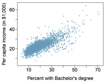
In many countries, there is a linear correlation between income and education level. On average, individuals with higher levels of education tend to earn more income.

• Nonlinear: cannot be accurately represented by a straight line.

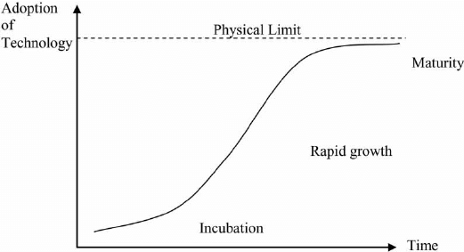
Example : Technology Adoption

The adoption of new technologies often follows an S-shaped (sigmoid) curve. Initially, adoption is slow, then it accelerates rapidly, and finally, it slows down again as the technology becomes ubiquitous. This is a classic example of a nonlinear trend.

Pearson correlation

Pearson correlation, also known as the Pearson correlation coefficient or Pearson’s r, is a statistical measure used to assess the strength and direction of the linear relationship between two continuous variables. It’s widely used in various fields, including economics, social sciences, and data analysis.

Definition: Pearson correlation quantifies how two variables move together. It provides a number between -1 and 1, where:

• 1 indicates a perfect positive linear relationship: As one variable increases, the other also increases at a constant rate.
• -1 indicates a perfect negative linear relationship
• 0 indicates no linear relationship

Assumptions:

• Pearson correlation assumes that the relationship between variables is linear.
• It also assumes that the variables follow a roughly normal distribution.

Formula: The formula for Pearson correlation between two variables X and Y with n data points is:

\[r = \frac{\sum{(X_i - \bar{X})(Y_i - \bar{Y})}}{\sqrt{\sum{(X_i - \bar{X})^2}\sum{(Y_i - \bar{Y})^2}}}\]

Where:

• \(X_i\) and \(Y_i\) are individual data points.
• \(\bar{X}\) and \(\bar{Y}\) are the means (averages) of \(X\) and \(Y\), respectively.

Causality: Exploring Cause-and-Effect Relationships

Causality refers to a relationship between two variables where changes in one variable directly influence or cause changes in another variable.

Establishing causality is a more complex endeavor than identifying correlation. While correlated variables might change together, it does not necessarily mean that changes in one variable are causing changes in the other.

To establish causality, researchers often need to conduct controlled experiments, observational studies, or employ advanced statistical techniques such as causal inference models.

=> Correlation does not necessarily imply causality.

Example: Ice Cream Sales and Drowning Incidents

Source: https://andreasrmadsen.medium.com/

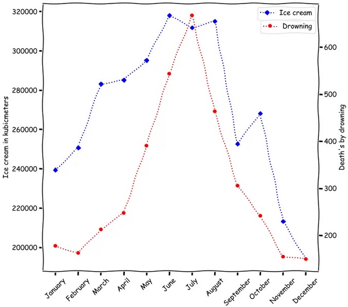
Imagine you’re a researcher examining data on ice cream sales and the number of drowning incidents at a beach over several months. You notice a strong positive correlation between the two variables, meaning that when ice cream sales go up, the number of drowning incidents tends to increase as well. You might be tempted to conclude that eating more ice cream somehow causes more drownings or vice versa.

However, this is a classic case of where correlation does not imply causality. In reality, there’s no direct causal relationship between eating ice cream and drowning. The apparent correlation can be explained by a hidden third variable: the weather, specifically, hot summer weather.

Here’s how it works:

1. Hot Weather: During the summer months, when the weather is hot, people are more likely to buy ice cream to cool off, and they’re also more likely to go swimming at the beach.

2. Increased Beach Activity: The hot weather leads to an increase in beach activity, including more people swimming in the water.

3. Drowning Incidents: With more people swimming, there’s a higher likelihood of drowning incidents occurring simply because there’s a larger pool of individuals exposed to the risk of drowning.

In this scenario, both ice cream sales and drowning incidents are independently influenced by the hot weather. There’s no direct causal link between eating ice cream and drowning; instead, they are correlated because they share a common cause.

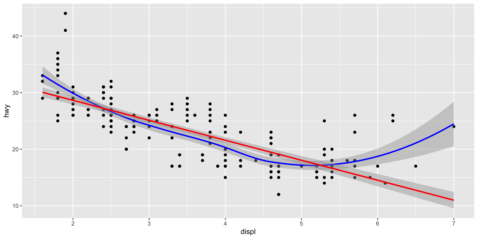
Before Exercise 1

Correlations

dataset <- data.frame(X = c(1, 2, 3, 4, 5, 6),
                      Y = c(2, NA, 5, NA, 4, 7),
                      Z = c(NA, 4, 6, NA, 8, 8))
dataset

  X  Y  Z
1 1  2 NA
2 2 NA  4
3 3  5  6
4 4 NA NA
5 5  4  8
6 6  7  8

• use = "everything" (default) includes all variables in the correlation matrix, treating missing values as NA.

cor(dataset, use = "everything")

   X  Y  Z
X  1 NA NA
Y NA  1 NA
Z NA NA  1

• use = "complete" excludes variables with any missing values from the correlation matrix.

cor(dataset, use="complete")

          X         Y         Z
X 1.0000000 0.5000000 0.9449112
Y 0.5000000 1.0000000 0.1889822
Z 0.9449112 0.1889822 1.0000000

d = dataset[apply(!is.na(dataset),1,all),c("X","Y")]
d

  X Y
3 3 5
5 5 4
6 6 7

cor(d, use = "everything")

    X   Y
X 1.0 0.5
Y 0.5 1.0

• use = "pairwise" maximizes the use of available data for each pair of variables, making the most of the available information.

cor(dataset, use="pairwise")

          X         Y         Z
X 1.0000000 0.8304819 0.9534626
Y 0.8304819 1.0000000 0.1889822
Z 0.9534626 0.1889822 1.0000000

d = dataset[,c("X","Y")]
cor(d, use = "complete")

          X         Y
X 1.0000000 0.8304819
Y 0.8304819 1.0000000

d2 = d[apply(!is.na(d),1,all),c("X","Y")]
d2

  X Y
1 1 2
3 3 5
5 5 4
6 6 7

cor(d2, use = "everything")

          X         Y
X 1.0000000 0.8304819
Y 0.8304819 1.0000000

geom_smooth

Linear or Non-linear correlations

library(ggplot2)
ggplot(mpg, aes(displ, hwy)) +
  geom_point() +
  geom_smooth(color="blue")+
  geom_smooth(method="lm", color="red")

Homework for next week

• Finish Exercise 1 (Social democratic capitalism)

• 1 application exercise about correlation

  • Search for help online (e.g. StackOverflow, more than ChatGPT)
  • be persistent (you will need it) and do your best!

• Handbooks, videos, cheatsheets

  • 2 chapters of Gerring and Christenson’s handbook (ch.20 and beginning of ch.21)