Comparison: Exploring Differences and Similarities
Comparison involves examining the differences or similarities between two (or more) distinct groups or categories.
- of Means: Analyzing the differences in the average values of different variables across distinct groups (t-test).
- of Proportions : Analyzing the differences in proportions or percentages between different groups (useful when dealing with categorical data, when examining the distribution of certain attributes across different categories) (chi-squared tests).
Ingredient 1: Estimation
Utilizing techniques to infer characteristics of a population from the information available in a sample.
Distribution
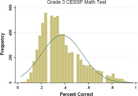
Illustrates the way data values are spread out or organized:
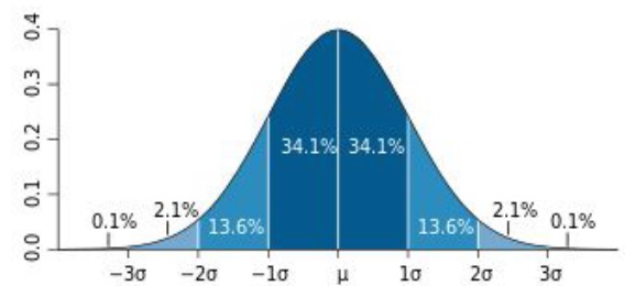
- normal distribution (bell-shaped curve),
- binomial distribution (often associated with binary outcomes such as counting successes in a fixed number of trials)
- …
Each type of distribution describes how data behaves under specific conditions.
Imagine you have a set of data, like the test scores of your classmates. A distribution is a way to describe how these scores are spread out or organized. It tells you the different values that the scores can take and how often each value appears.
Example: If you have 30 test scores in your class, a distribution might show that 5 students scored 90, 10 students scored 80, 8 students scored 70, and so on.
![]()
Mathematical Foundations
They validate the reliability of estimation techniques:
Law of Large Numbers: This principle states that as the size of a sample increases, the estimate of the population parameter becomes more accurate.
Central Limit Theorem: The distribution of sample means approaches a normal distribution as the sample size increases, irrespective of the shape of the population distribution.
This theorem is a powerful tool that enables statisticians to make inferences about population parameters even when the population distribution is unknown or non-normal.
Ingredient 2: Test Statistics
It tests the presence of a relationship between variables.
t-test (parametric)
It determines whether the observed difference between the means of a variable of two groups is statistically significant. It relies on the Student’s t-distribution.
Chi-squared test (nonparametric)
It is used to analyze the association / independence between categorical variables. It compares observed frequencies to expected frequencies in a contingency table. It relies on the Chi-squared distribution.
Null Hypothesis (\(H_0\))
It is a statement that suggests, for example, that there is no significant relationship between the variables being studied (default assumption).
p-values
A measure of compatibility with the null hypothesis; values lower than a threshold (e.g., p < 0.05) lead to the rejection of the null hypothesis.
Confidence Intervals
Provides a range of values that you use to estimate a population parameter (like the average test score of all students) based on a sample of data.
A confidence interval helps you estimate something about a larger group based on what you’ve seen in a smaller group, and it gives you a sense of how confident you can be in that estimate.
Example: Suppose you have a sample of the test scores for 30 students, and you want to estimate the average test score for all students in your school. You calculate a confidence interval, which might say, “We are 95% confident that the average test score for all students in the school falls between 10 and 11/20.
If you were to take many different random samples and calculate confidence intervals from them, about 95% of those intervals would contain the true population parameter.
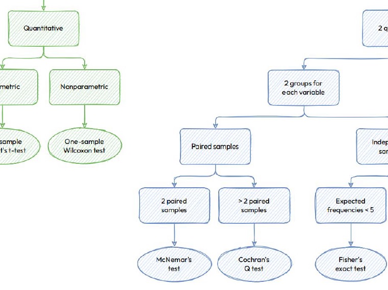
There are many significance tests
The choice of which test to use depends on factors such as the nature of the data, the number of groups being compared, and the assumptions underlying each test. It’s essential to understand the characteristics of your data and the requirements of each test to select the most appropriate one for your analysis.


