library(dplyr)10 Logistic Regression
Session 10
By the end of this session, you have learned more about non linearity in dependent variables and how to explore generalized linear regression (GLM) as one of the fundamental tools in data analysis and statistics, in particular to predict a yes/no dependent variable
In a nutshell
- capabilities of generalized linear models
- In practice you have learned to:
- Interpret the parameters of a generalized linear model with the example of binomial law (logit), which involves understanding the coefficients and their implications for the relationships between variables.
- Comparing models with AIC and BIC indicators.
10.1 Non-linearity
Feedback about Exam 1
- Structure of code nearly perfect :
install.packagesin comments.setwdOUTSIDE thedatafolder
select,group_by,mutatemastered in all groups- Don’t forget to explain each step (
paste0,as.Dateorwdaysometimes forgotten) - Q8 and Q9 not right for everybody
➡️ All marks are > 15/20. BRAVO! But next exams will be more challenging 😳
10.1.1 Non linearity for variables
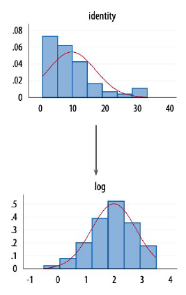
Variables that violate model assumptions will often do so due to high skewness (non symetric distribution)
A possible fix might be to transform the scale on which those variables are measured.
Often:
- logarithmic transformation (predictor will have a quadratic effect on the dependent variable)
- square transformation (more complex to interpret)

10.1.2 Logarithmic coefficients
linear relationship (last week) \[Y = \alpha + \beta X\]
log-linear relationship \[ln Y = \alpha + \beta X\]
lin-log relationship \[Y = \alpha + \beta ln X\]
log-log relationship \[ln Y = \alpha + \beta ln X\]
An increase in 1 unit of \(X\) is associated with an increase of \(\beta\) unit in \(Y\)
An increase in 1 unit of \(X\) is associated with a \(100 \ \beta\%\) change in \(Y\)
A \(1\%\) increase in \(X\) is associated with a \(0.01 \ \beta\%\) change in \(Y\)
A \(1\%\) increase in \(X\) is associated with a \(\beta\%\) change in \(Y\)
10.2 Generalized Linear Models (GLM)
10.2.1 Nonlinearity for models
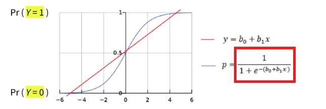
When dealing with a binary dependent variable (\(Y = 0\) or \(Y = 1\)), logistic regression is commonly used.
In logistic regression, we introduce a link function to model the relationship between the predictor(s) and the binary response variable.

It allows to express the relationship between Y and its predictor(s) through a linear model, at the price of having to interpret that relationship through log-odds, which can be converted into probabilities of \(P(Y = 1)\) through exponentiation (see after).
10.2.2 Logistic regression coefficients
Logistic regression equation
\[L = \underbrace{ln (\frac{p}{1-p})}_\text{= log-odds = logit } = \alpha + \beta X \qquad\text{ or } \qquad p = \frac{e^{\alpha + \beta X}}{1 + e^{\alpha + \beta X}}\]
with
- \(p = P(Y = 1)\)
- \(\ln\) : natural logarithm.
- \(X\) is the predictor variable.
- \(\alpha\) is the intercept.
- \(\beta\) is the coefficient associated with the predictor variable.
Interpretation : odd-ratios
\[\text{Odds Ratio} = e^\beta\]
For 1-unit increase in \(X\), \(P(Y = 1)\) increase by a factor of \(e^\beta\).
- \(OR > 1\) denotes a higher probability of Y = 1 (OR = 1.24 denotes a 24% increase)
- \(OR < 1\) denotes a lower probability of Y = 1 (OR = 0.5 denotes \(P(Y=1)\) divided by 2)
10.3 Before Exercise 1
Testing for the presence of the bacterium H. influenzae (y) in children based on the administration of a medication versus a placebo (trt). The presence of the virus was monitored at weeks 0, 2, 4, 6, and 11 (week).
utils::data(bacteria, package = "MASS")
str(bacteria)
'data.frame': 220 obs. of 6 variables:
$ y : Factor w/ 2 levels "n","y": 2 2 2 2 2 2 1 2 2 2 ...
$ ap : Factor w/ 2 levels "a","p": 2 2 2 2 1 1 1 1 1 1 ...
$ hilo: Factor w/ 2 levels "hi","lo": 1 1 1 1 1 1 1 1 2 2 ...
$ week: int 0 2 4 11 0 2 6 11 0 2 ...
$ ID : Factor w/ 50 levels "X01","X02","X03",..: 1 1 1 1 2 2 2 2 3 3 ...
$ trt : Factor w/ 3 levels "placebo","drug",..: 1 1 1 1 3 3 3 3 2 2 ...bacteria <- bacteria %>%
mutate(y = factor(ifelse(y=="n",0,1), levels=c(0,1)))In mean, bacteria presence decreases with time
prop.table(table(bacteria$week,bacteria$y),1)
              0          1
  0  0.10000000 0.90000000
  2  0.09090909 0.90909091
  4  0.26190476 0.73809524
  6  0.27500000 0.72500000
  11 0.27272727 0.72727273
In mean, bacteria presence decreases thanks to drugs
prop.table(table(bacteria$trt,bacteria$y),1)
                  0         1
  placebo 0.1250000 0.8750000
  drug    0.2903226 0.7096774
  drug+   0.2096774 0.7903226
Fit models (most parsimonious to full).
GLM0 <- glm(y ~ 1, data = bacteria, family = binomial(link = "logit"))
GLM1 <- glm(y ~ week, data = bacteria, family = binomial(link = "logit"))
GLM2 <- glm(y ~ trt + week, data = bacteria, family = binomial(link = "logit"))
Note: If you forget to specify family = binomial in the glm function for a binary response variable (i.e., a binary logistic regression), the default family assumed is family = gaussian, which corresponds to linear regression.
Compare them.
texreg::screenreg(list(GLM0, GLM1, GLM2))
=====================================================
                Model 1      Model 2      Model 3
-----------------------------------------------------
(Intercept)        1.41 ***     1.96 ***     2.55 ***
                  (0.17)       (0.29)       (0.41)
week                           -0.11 *      -0.12 **
                               (0.04)       (0.04)
trtdrug                                     -1.11 **
                                            (0.43)
trtdrug+                                    -0.65
                                            (0.45)
-----------------------------------------------------
AIC              219.38       214.91       211.81
BIC              222.77       221.70       225.38
Log Likelihood  -108.69      -105.45      -101.90
Deviance         217.38       210.91       203.81
Num. obs.        220          220          220
=====================================================
*** p < 0.001; ** p < 0.01; * p < 0.05
GLM2 (Model 3) minimizes AIC and seems to be the best model.
Exponentiate GLM2 coefficients to read log-odds.
broom::tidy(GLM2, exponentiate = TRUE)# A tibble: 4 × 5
term estimate std.error statistic p.value
<chr> <dbl> <dbl> <dbl> <dbl>
1 (Intercept) 12.8 0.406 6.28 3.42e-10
2 trtdrug 0.331 0.425 -2.60 9.25e- 3
3 trtdrug+ 0.521 0.446 -1.46 1.44e- 1
4 week 0.891 0.0441 -2.62 8.72e- 3For 1-unit increase in
week, \(P(Y = 1)\) is divided by1/0.89 = 1.12.Taking resp. drug/drug+ instead of a placebo, \(P(Y = 1)\) is divided by 3 and 2.
Exam 2
- Instructions here
- in group & graded (like Exam 1)
- same real-world dataset (road traffic accidents in France)
- data visualisation and data analysis (correlation, link between variables) tasks
- Submit a script called
exam2_solution.R(Subject : “DSR Exam 2 Submission”, To : kim.antunez@sciencespo.fr) - Deadline : apr. 30th, before 7:15 pm.
- Make sure your script is well-organized (you all did well last time)